UNIT 2
Theory of cost
The traditional theory of costs analyses the behavior of cost curves in the short-run and long-run and arrives at the conclusion that both the short-run and long-run cost curves are U-shaped but the long-run cost curves are flatter than short-run cost curves.
Short run cost of the traditional theory
In the traditional theory of the firm, in the short run, there are variable inputs and at least one fixed input. This suggests that short run costs are divided into fixed costs and variable costs. Thus, there are three concepts of total cost in the short run: Total fixed costs (TFC), total variable costs (TVC), and total costs (TC).
TC = TFC + TVC
- In the words of Ferguson, “Total fixed cost is the sum of the ‘short run explicit fixed costs and implicit costs incurred by the entrepreneur.”

2. Total variable cost
According to Ferguson, “total variable cost is the sum of amounts spent for each of the variable inputs used”

In the above figure, TVC changes with the change in the level of production
3. Total cost

4. Average fixed cost (AFC)–

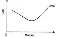
5. Average variable cost (AVC)
6. Average cost of production (AC)

7. Marginal cost (MC)

Proportionate change in output

Long run cost
In long run, all the factors of production vary. Long run is period in which all cost change as all the factors of production are variable. To produce at a lower cost in long run, the organization should have the ability to change the factors of production. There is no difference between TC and TVC as there is no fixed cost.
- It refers to the minimum cost at which a given level of output can be produced.
- Definition
According to Leibhafasky, “the long run total cost of production is the least possible cost of producing any given level of output when all inputs are variable.”

2. Long run average cost (LAC)

3. Long run marginal cost (LMC)-
Modern theory of cost
The Modern theory suggests the existence of ‘built- in- reserve capacity ‘which imparts flexibility and enables the plant to produce larger output without adding to the costs. Built –in- reserve capacity are planned by firms. Modern theory of costs does not agree with the U-shape of the cost curves. The short-run cost curve has a saucer- type shape whereas the long-run Average cost curve is either L-Shaped or inverse J-shaped.
According to the Modern theory of costs,the firm can produce a range of output and not a single level of output as under the traditional theory of cost. Firms build industrial plants with some flexibility in their productive capacity so that instead of a single output level, there is a whole range of output that can be produced optimally at low cost. The ‘Built-in Reserve capacity’ provides ‘maximum flexibility’ in the production process. The Planned reserve capacity explains the ‘Saucer – shaped’ short run average variable costs.
The Modern theory of cost stresses on the role of economies of scale, which significantly enables the firm to continue production at the lowest point of average cost for a considerable period of time. The firm checks diseconomies of scale by planning in advance and enjoys the gains of production in comparison to the traditional theory where the average cost rises after the firm reaches the optimal level of output. Developments in managerial economies explain the L – Shaped and inverse J –Shaped LAC Curves.
Short run cost curve
The short-run Average costs consist of the Average fixed costs and Average variable costs. Because of the U- shaped AVC curve under the traditional theory, the Plant is designed to optimally produce a single level of output (at the minimum point of AVC CURVE) . In case there is any departure from the optimizing output, there arises an excess capacity or unplanned capacity.
If the firm produces a lower level of output OX1 then costs would be high compared to OXm level of output. The short- run Average variable costs (SAVC) has a Saucer-type shape where there is a flat- stretch corresponding to the ‘RESERVE CAPACITY ‘ or the ‘PLANNED CAPACITY ‘ – which the Plant builds to provide flexibility in the firm’s production process.

Long run cost curve
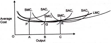
All costs are variable in the long run and they give rise to a long run cost curve which is roughly L-shaped. Empirical evidence about the long run average cost curve reveals that the LAC curve is L-shaped rather than U-shaped. In the beginning, the LAC curve rapidly falls but after a point, “the curve remains flat, or may slope gently downwards, at its right-hand end”. Production cost fall continuously with increases in output. At very large scales of output, managerial costs may rise. But the fall in production costs more than offsets the increase in the managerial costs, so that the total LAC falls with increases in scale. Economists have assigned the following reasons for the L-shape of the LAC curve.

Each SAC curve includes production costs, managerial costs, other fixed costs and a margin for normal profits. Each scale of plant (SAC) is subject to a typical load factor capacity so that points A, B and C represent the minimal optimal scale of output of each plant. By joining all such points as A, B and C of a large number of SACs, we trace out a smooth and continuous LAC curve, as shown in below Figure

2. Technical progress: Another reason for the existence of the Lshaped LAC curve in the modern theory of costs is technical progress. The traditional theory of costs assumes no technical progress while explaining the U-shaped LAC curve. The empirical results on long-run costs confirm the widespread existence of economies of scale due to technical progress in firms. The period, between which technical progress has taken place, the long-run average costs show a falling trend. The evidence on diseconomies is much less certain. So an upturn of the LAC at the top end of the size scale has not been observed. The L-shape of the LAC curve due to technical progress is explained in Figure above.
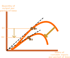
Suppose the firm is producing 0Q1 output on LAC1 curve at per unit cost of 0C1 output on LAC1 curve at a per unit cost of 0C1. If there is an increase in demand for the firm's product to 0Q2, with no change in technology, the firm will produce 0Q2 output along the LAC1 curve at per unit cost of 0C'. If, however, there is technical progress in the firm, it will install a new plant having LAC2 as the long-run average cost curve. On this plant, it produces 0Q2 output at a lower cost 0C2 per unit. Similarly, if the firm decides to increase its output to 0Q3 to meet further rise in demand, technical progress may have advanced to such a level that it installs the plant with the LAC3 curve. Now it produces 0Q3 output at a still lower cost 0C3 per unit. If the minimum points, L, M and N of these U-shaped long-run average cost curves LAC1, LAC2 and LAC3 are joined by a line, it forms an L-shaped gently sloping downward curve LAC.
3. Learning: Yet another reason for the L-shaped long-run average cost curve is the learning process. Learning is the product of experience. If experience in this context can be measured by the amount of a commodity produced, then higher the production is, the lower it is per unit cost. The consequences of learning are similar to increasing returns. First, the knowledge gained from working on a large scale cannot be forgotten. Second, learning increases the rate of productivity. Third, experience is measured by the aggregate output produced since the firm first started to produce the product. Learning by doing has been observed when firm starts producing new products. After they have produced the first unit, they are able to reduce the time required for production and thus reduce per unit cost.
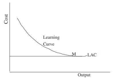
Figure shows a learning curve (LAC) which relates the cost of producing a given output to the total output over the entire time period. Growing experience with making the product leads to falling costs as more and more of it is produced. When the firm has exploited all learning Cost Learning Curve LAC LMC possibilities, costs reach a minimum level, M in the figure. Thus the LAC curve is L-shaped due to learning by doing.
Key takeaways –
2. Modern theory of cost curves has been propounded by economists like Stigler, Andrews etc. According to traditional theory of cost curves, cost curves are U-shaped. But according to modern theory, in real life, cost curves are L-shaped.
Production function
To have clear knowledge about production and cost it’s mandatory to know the basics of production functions and understand the fundamentals in mathematical terms. We break down short-term and long-term production functions supported variable and glued factors.
What is the production function?
The functional relationship between the physical input (or factor of production) and therefore the output is named a production function. It assumed the input as an explanatory or independent variable and the output as a dependent variable. Mathematically, you can write this as:
Q=f (L, K)
Where "Q" represents the output, "L" and "K" are the inputs, respectively, labour and capital (such as machinery). Note that there may be many other factors, but we are assuming a two-factor input here. Production functions are defined differently in the short term and in the long term. This distinction is crucial in microeconomics. This distinction is based on the nature of the factor input.
Inputs that change directly with the output are called variable factors. These are factors that can change. Fluctuating factors exist both in the short term and in the long term. Examples of variable factors include daily labour and raw materials.
On the other hand, factors that cannot change or change as the output changes are called fixed factors. These factors are usually characteristic only for a short or short period of time. There are no fixed factors in the long term.
Therefore, two production functions can be defined: short-term and long-term. A short-term production function defines the connection between one variable factor (keeping all other factors fixed) and therefore the output. The law of regression to factors explains such a production function.
For example, suppose that a company has 20 units of Labour and 6 acres of land, and initially uses only Labour units (variable coefficients) for that land (fixed coefficients). Thus, the ratio of land and labour is 6: 1. Now, if the company chooses to adopt 2 labour units, then the ratio of land to Labour will be 3: 1 (6: 2).
Here, all factors change in the same proportion. The law used to explain this is called the law of return to scale. It measures how much of the output changes when the input changes proportionally.
Key takeaways –
Law of Variable Proportions
The law of variable proportion states that keeping all other factors fixed, when the quantity of one factor increased, the marginal product of that factor will eventually decline. This means that upto the use of a certain amount of variable factor, marginal product of the factor may increase and after a certain stage it starts diminishing. When the variable factor becomes relatively abundant, the marginal product may become negative.
Definition
“As the proportion of the factor in a combination of factors is increased after a point, first the marginal and then the average product of that factor will diminish.” Benham
Assumption
The following assumption of law of variable proportion
Illustration of the Law:
The law of variable proportion is explained in the below given table and figure. Assume that a there is a given fixed amount of land, in which more labour (variable factor) is used to produce agricultural product.
Units of labour | Total product | Marginal product | Average product |
1 | 2 | 2 | 2 |
2 | 6 | 4 | 3 |
3 | 12 | 6 | 4 |
4 | 16 | 4 | 4 |
5 | 18 | 2 | 3.6 |
6 | 18 | 0 | 3 |
7 | 14 | -4 | 2 |
8 | 8 | -6 | 1 |
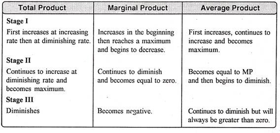
In the above table we can observe that upto the use of 3 units of labour, total product increases at an increasing rate. But after the third unit total product increases at a diminishing rate.
A marginal product is the incremental change in total product as a result of increasing the variable factor i.e labour. We can see from the table, marginal product of labour initially rises and beyond the use of third unit it starts diminishing. The use of 6 units does not add anything in the production. Thus marginal product of labour fallen to zero. After the 6 unit, total product decreases and marginal product becomes negative.
Average product is derived by dividing total product by the quantity of variable unit. Till the 3 unit of labour, average product increases. Whereas after the 3 unit, average product is falling throughout.
Three Stages of the Law of Variable Proportions:
The stages are discussed in the below figure where labour is measured on the X-axis and output on the Y-axis.
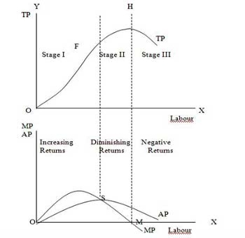
Stage 1. Stage of Increasing Returns:
In this stage, total product increases at an increasing rate till point F..ie the curve TP concave upwards upto point F which means marginal product of labour rises. Because efficiency of fixed factor increases with the increase in variable facto labour. After point F, the total product starts increasing at a diminishing rate. Looking at the next figure, marginal product of labour is maximum, after which it diminishes. This stage is called the stage of increasing returns because the average product of the variable factor labour increases throughout this stage. This stage ends at the point where the average product curve reaches its highest point.
Stage 2. Stage of Diminishing Returns:
The stage 2 ends, when the total product increases at a diminishing rate until it reaches it maximum point H. In this stage both marginal product and average product are diminishing but remain positive. Because fixed factor land becomes inadequate with the increase in the quantity of variable factor labour. At point M marginal product is zero which corresponds to the maximum point H of the total product curve.
Stage 3. Stage of Negative Returns:
In stage 3, with the increase in variable factor labour, the total product decline. Therefore the TP curve slopes downward. As a result, marginal product of labour is negative and MP cure falls below x axis. In this case fixed factor land becomes too much inadequate to the increase in variable factor labour.
Key takeaways –
Law of Returns to Scale
In long run, no factors are fixed. Return of scale refers to proportionate change in productivity from proportionate change in all the inputs.
Definition:
“The term returns to scale refers to the changes in output as all factors change by the same proportion.” Koutsoyiannis
“Returns to scale relates to the behaviour of total output as all inputs are varied and is a long run concept”. Leibhafsky
Types of return of scale
1. Increasing return of scale
2. Constant return of scale
3. Diminishing return of scale
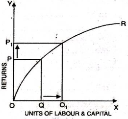
Explanation
- When proportionate increase in factors of production leads to higher proportionate increase in production refers to increasing return of scale.
- In the below figure, x axis represent increase in labour and capital while Y axis represent increase in output. When labour and capital increases from Q to Q1, output also increases from P to P1 which is higher than the change in factors of production ie labour and capital

2. Diminishing return of scale
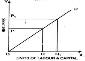
3. Constant return of scale
Key takeaways –
Internal and external economies and diseconomies
Economies of scale are the factors which reduces the production cost as the volume of output increases. This means firm produces more output, then marginal cost of production decreases.
Economies of scale is divided into internal and external
3. Managerial economies of scale - the employment of specialised workforce result in managerial economies of scale. As the organisation grow, they hire more expert staff and create a specialised business unit. The firm efficiency is increased by employing specialist, accountants, human resource, etc which will result in reducing the cost of production and increase revenue.
4. Marketing economies of scale – marketing economies of scale is the ability to spread advertising and marketing budget over an increasing output. As the production increases the firm can fix marketing expenses, which will reduce the per unit cost of production. Better advertisement result in reaching larger audience and increase the sale of the firm.
5. Financial economies of scale – access of financial and capital market result in financial economies of scale. Large firms find easier and cheaper to raise funds. As the firm grow, it is considered to be more credit worthy. They can easily raise fund from banks, stock markets.
6. Commercial economies of scale – reduction in price due to discounts or bargaining power result in commercial economies of scale. Larger firms can buy goods and services in larger quantities. Thus they get larger discount and can bargain to negotiate lower prices. This means they pay less for each item purchases.
7. Network economies of scale - when the marginal costs of adding additional customers are extremely low result in network economies of scale. This means larger firm can support large numbers of new customers with their existing infrastructure can substantially increase profitability as they grow.
External economies of scale – external economies of scale are caused by changes outside the firm but within the industry. The factors affect the whole industry. four different types of external economies of scale: (1) infrastructure, (2) supplier, (3) innovation, and (4) lobbying economies of scale.
2. Specialization economies of scale – when suppliers and workers focus on a particular industry due to its size result in specialization economies of scale. When company within the industry increases its size and numbers, suppliers focus in that particular industry. Similarly, similarly workers find job in those industry which is growing in size.
3. Innovation economies of scale – increases public and private research result in innovation economies of scale. Industries have significant impact on the society result in growing public interest. This allows them to collaborate with research facilities and university to improve their products and processes
4. Lobbying economies of scale - Lobbying economies of scale arise from an increase in bargaining power as industries become more significant. The government is ready to compromise as these industry provide a lot of jobs and pay a significant amount of taxes.
Uneconomics of scale occurs when the long-term average cost of an organization increases. It can occur when the tissue becomes excessively large. In other words, uneconomics of Scale Causes larger org-anizations to produce goods and services at increased costs.
There are two types of scale diseconomies: internal diseconomies and external diseconomies, which are discussed as follows:
See uneconomical raising the cost of production in the organization. The main factors affecting the cost of production of the organization include the lack of determination, supervision and technical difficulties.
2. External uneconomics of the scale:
See uneconomical to limit the expansion of an organization or industry. Factors acting as restraints on expansion include increased production costs, a shortage of raw materials and a decline in the supply of skilled workers.
There are several causes of diseconomics of scale.
Some of the causes that lead to uneconomics of scale are:
If the organization's production goals and objectives are not properly communicated to employees in the organization, they can lead to overproduction or production. This can lead to diseconomics of scale.
Separately, if the communication process in the organization is not strong, then the employee will not get enough feedback. As a result, there will be less face-to-face interaction between employees, which will affect the production process.
This leads to a decrease in productivity levels. For large organizations, workers may feel isolated and less motivated because they are less valued for their work. Because of poor communication networks, it is difficult for employers to interact with employees and build a sense of attributes. This leads to a decrease in the productivity level of output due to lack of motivation. This further leads to an increase in the cost of the organization.
It serves as the main problem of large organizations. Monitoring and controlling the work of all employees in a large organization becomes impossible and expensive. It is difficult to make sure that all employees of the organization are working towards the same goal. It becomes difficult for managers to direct the sub-coordinates of large organizations.
It means a situation where an organization is facing competition from its products. While smaller organizations face competition from the products of other organizations, larger organizations find their products compete with each other.
References


