UNIT 4
Production
Marginal productivity theory
The oldest and most significant theory of factor pricing is the marginal productivity theory. It is also known as Micro Theory of Factor Pricing.
It was propounded by the German economist T.H. Von Thunen. But later on, many economists like Karl Mcnger, Walras, Wickstcad, Edgeworth and Clark etc. contributed for the development of this theory.
“The distribution of income of society is controlled by a natural law, if it worked without friction, would give to every agent of production the amount of wealth which that agent creates.” -J.B. Clark
“The marginal productivity theory contends that in equilibrium each productive agent will be rewarded in accordance with its marginal productivity.” -Mark Blaug
Assumptions of the Theory:
The main assumptions of the theory are as under:
Perfect Competition:
The marginal productivity theory rests upon the fundamental assumption of perfect competition. This is because it cannot take into account unequal bargaining power between the buyers and the sellers.
Homogeneous Factors:
This theory assumes that units of a factor of production are homogeneous. This implies that different units of factor of production have the same efficiency. Thus, the productivity of all workers offering the particular type of labour is the same.
Rational Behaviour:
The theory assumes that every producer desires to reap maximum profits. This is because the organizer is a rational person and he so combines the different factors of production in such a way that marginal productivity from a unit of money is the same in the case of every factor of production.
Perfect Substitutability:
The theory is also based upon the assumption of perfect substitution not only between the different units of the same factor but also between the different units of various factors of production.
Perfect Mobility:
The theory assumes that both labour and capital are perfectly mobile between industries and localities. In the absence of this assumption the factor rewards could never tend to be equal as between different regions or employments.
Interchangeability:
It implies that all units of a factor are equally efficient and interchangeable. This is because different units of a factor of production are homogeneous, since they are of the same efficiency, they can be employed inter-changeable, and e.g., whether we employ the fourth man or the fifth man, his productivity shall be the same.
Perfect Adaptability:
The theory takes for granted that various factors of production are perfectly adaptable as between different occupations.
Knowledge about Marginal Productivity:
Both producers and owners of factors of production have means of knowing the value of factor’s marginal product.
Full Employment:
It is assumed that various factors of production are fully employed with the exception of those who seek a wage above the value of their marginal product.
Law of Variable Proportions:
The law of variable proportions is applicable in the economy.
The Amount of Factors of Production should be Capable of being Varied:
It is assumed that the quantity of factors of production can be varied i.e. their units can either be increased or decreased. Then the remuneration of a factor becomes equal to its marginal productivity.
The Law of Diminishing Marginal Returns: It means that as units of a factor of production are increased the marginal productivity goes on diminishing.
Long-Run Analysis:
Marginal productivity theory of distribution seeks to explain determination of a factor’s remuneration only in the long period.
Modern theory
The marginal productivity theory, only tells us how many workers will an employer engage at a given wage-level in order to maximise his profit.
The modern theory of factor pricing which provides satisfactory explanation of factor prices is the Demand and Supply Theory. Just as the price of a commodity is determined by the demand for, and supply of, a commodity, similarly the price of a productive service also is determined by demand for, and supply of, that particular factor.
Demand for a Factor:
Let us first consider the demand side. In the first place, we should remember that the demand for a factor of production is not a direct demand if is an indirect or derived demand. It is derived from the demand for the produce that the factor produces. For instance, labour does not satisfy our wants directly. We want labour for the sake of the goods that it produces. It follows, therefore, that if the demand for goods increases, the demand for the factors which help to produce these goods will also increase. Also, if the demand for goods is elastic or inelastic, the demand for the factors too will be elastic or inelastic.
The demand for a factor of production will also depend on the quantity of the other factors required in the process. Generally speaking, the demand price for a given quantity of a factor of production will be higher, the greater the quantities of the co-operating productive services. If more of a factor of production is employed, the marginal productivity of the factor will fall, and the lower will be the demand price for the unit of a productive service. This is another rule connected with the demand for a factor of production.
The demand price of a factor of production also depends on the value of the finished product in the production of which the factor is used. The demand price will generally be greater; the more valuable is the finished product in which the factor is used. Also, the more productive the factor, he higher will be the demand price of a given quantity of the factor.
These are a few points connected with the demand for a productive service. We know that the demand curve of the industry is the sum-total of the demand curves of the various firms in the industry. By a similar summing up, we can have the demand curve of all the industries using a particular productive service.
The demand of the employer for a factor depends on its marginal revenue productivity (in short, marginal productivity), and the quantity of the factor that a firm will employ will depend on the prevailing wage-level. That is more labour will be employed if wages are low and less if wages are high.
In the below figure (a) illustrates the position of a firm regarding the employment of a factor, say, labour. When the wage is OW, the firm is in equilibrium at the point E and the demand for the factor is ON; similarly, at OW’ wage, the demand is ON’, and at OW” the demand is ON”. MRP (marginal revenue productivity) curve is the demand curve for a factor of production by an individual firm.

But for determining the price of a factor, it is not the demand of the individual firm for it that matters. What matters is the total demand, i.e., the sum-total of the demands of all firms in the industry. The total demand curve is derived by the lateral summation of the marginal revenue productivity curves of all the firms. This curve DD is shown in the above Fig.(b).
It can be seen that Y-axes in both curves are drawn to the same scale, but X-axes are drawn on different scales. We have supposed that there are 100 firms in the industry. At OW wage, the demand of the individual firm is ON, but the demand of the whole industry at the same wages is OM, which is equal to 100 ON (because the number of firms in the industry is 100). In the same manner, at OW’ the demand of the firm is ON’ but of the entire industry OM’, which is equal to 100 ON’, and at OW”, the demand of the firm is ON” and that of the industry OM”, which is equal to 100 ON”.
It can be seen that the demand curve DD slopes downward to the right. The reason is that MRP curve, whose summation is represented by DD, also slopes down similarly to the right in the relevant portion. This means that according to the law of diminishing marginal productivity, the more a factor is employed the lower is the marginal productivity. This is all about the demand side.
Supply Side:
As for the supply side, the supply curve of a factor depends on the various conditions of its supply. Take the case of labour—a very important productive service. The supply of labour will depend on the size and composition of population, its occupational and geographical distribution, labour efficiency, cost of education and training, cost of movement, the expected income, relative preference for work and leisure, and so on. In this manner, by considering all the relevant factors, it is possible to construct the supply curve of a productive service.
At the same time, we must note that the supply is a bit of complicated thing. We generally say that the supply of land is limited. But the fact is that, although for the whole community land is limited, for a particular firm or an industry, its supply is not limited. The supply can be increased if higher rent is offered.
In the case of commodities, we see that generally an increase in price brings forth larger supplies. This, however, does not necessarily hold good in the case of the factors of production. It may happen in some cases that, if wags go up, labour may be able to satisfy its needs by working for less time than before. They may prefer leisure to work. In this case, when the price of factor (or its remuneration) is increased, the supply is reduced. This peculiarity will be represented by a backward sloping curve after a stage.
Also, the supply of labour does not merely depend on economic factors; many non-economic considerations also enter. All the same, we can say that, if the price of a factor increases, its supply will also generally increase, and vice versa. Hence, the supply curve of a factor rises from left to right upwards. This is shown in the below fig.
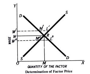
Interaction of Demand and Supply:
Now we have worked our way to the demand curve and the supply curve of a factor of production. Both these curves are needed for the determination of the price of a productive service. That price will tend to prevail in the factor market at which the demand and supply are in equilibrium. This equilibrium is at the point of intersection of the demand and supply curves.
In the second they intersect at the point R, and the price of the factor will be OW. At OW’ demand W’M’ is less than the supply W’L’. In this case, competition among the sellers of the service will tend to bring down the price to OW. On the other hand, at OW” price, the demand W”L” is greater than the supply W”M”; hence price will tend to go up to OW at which the demand and supply will be equal.
This is how the price of a factor of production in the factor market is determined by the interaction of the forces of demand and supply relating to that factor of production.
Key takeaways - The marginal product of a labour in any industry is the amount by which the output would be increased if a unit of labour was increased, while the quantities of other factors of production remaining constant.
Meaning
Wage is defined as the price paid for the services rendered by the labour in the production process. If wages are paid according to the amount or quantum of work done, it is called piece-wage. E.g. wage for weeding in one acre of paddy field. If wages are paid to a labour who works for a fixed period of time, it is known as time wage. E.g., wage for weeding per labour per day.
When payment is made in terms of cash or money, it is known as money wage or nominal wage. Real wage refers to the income of a worker in terms of real benefit. It refers to the amount of necessaries, comforts, and luxuries that a labour can obtain in return for his services. Real wage refers to the purchasing power of money earned by the labour or wages paid in terms of quantity of commodities. The standard of living of a labour depends on his real wage.
Determination of wage rate under perfect competition and monopoly
Under perfect competition, equilibrium wage rate is determined where demand for labour is equal to supply of labour.
In other words, under perfect competition, a labour will get wage equal to its marginal revenue productivity in the long run.
In the below fig units of labour have been measured on X-axis and wages on Y-axis. DD and SS are the demand and Supply curves of labours respectively. Both the curves intersect each other at point E which determines wage rate OP in the market.
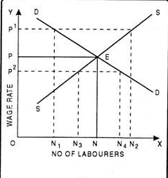
At this level of wages, ON units of labours will get employment. Now suppose, wages go up to OP1. At this price, demand is ON1 and supply ON2. Since, the supply is more than demand; it will lead to competition among labours to get employment which in turn results in a decrease in wage rate. On the other hand, if w age rate falls to OP2, demand will be more than the supply. This results in competition among the producers to get the services of labour which in turn leads to an increase in wage rate. Therefore, we may observe that equilibrium will be restored at that point where demand curve of labours intersects the supply curve of labours.
The study of firm’s equilibrium can be studied in the following two time periods:
1. Short Run
2. Long Run
1. Short Run Period:
Short run refers to a period in which it is not possible for a firm to fully equate the demand for and supply of a factor. Therefore, a firm in the short run may face three situations.
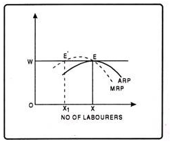
Supernormal Profit:
If at OW wage rate, a firm provides employment to as much labourers whose ARP is more than the prevailing wage, the firm earns supernormal profits. In the Fig a firm at its equilibrium provides employment to OX labourers. Here ARP i.e. PX is greater than the wage rate EX. Thus, firm earns EP as supernormal profits.

Normal Profit:
A firm enjoys normal profits, if ARP is equal to wage rate. In Fig when firm employs ON number of labours, their ARP is EX which is equal to prevailing wage rate OW. Thus, the firm gets only normal profits.

Losses:
A firm incurs losses, if at prevailing wage; a firm employs the number of labours at which their ARP is less than the prevailing wage rate. In Fig when firm employs OX labours, their ARP = PX is less than their wage rate OW. Thus, the firm has to incur losses equal to EP.

2. Long Run Period:
In the long run, a firm earns normal profit. A firm will be in equilibrium where ARP is equal to MRP. In Fig when firm employs OX labour ARP is equal to MRP.
Wage Determination under Imperfect Competition:
In the world of reality there exists imperfect competition rather than perfect competition. Therefore, Mrs. Joan Robinson and Prof. Pigou gave the wage rate determination under the conditions of imperfect competition.
The wage rate determination can be explained fewer than two heads:
(a) Perfect competition in product Market and Monopsony in the Labour market.
(b) Monopoly in the product Market and Monopsony in Labour Market.
(a) Perfect Competition in Product Market and Monopsony in Labour Market:
When there is a single buyer of labour in the market, monopsony is said to exist in the labour market. If there is an increase in monopolist’s demand for labour, wage rate will follow the same path which in turn tends to increase the average and marginal wage rate. It can be shown with the help of a diagram.
In Fig. units of labour have been measured on X-axis while wages on Y-axis. ARP and MRP is the average revenue product and marginal revenue product curves. AW and MW are the upward sloping average wage and marginal wage curves indicating that if the monopolist wishes to employ more and more labours, he has to offer the higher wage rate.
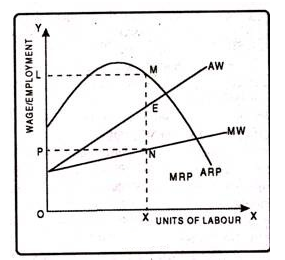
The monopolistic firm is in equilibrium at point E. At point E both the conditions of equilibrium are fulfilled i.e. marginal wage should be equal to marginal revenue product and the marginal revenue product curve must cut the marginal wage curve from above and then lies below it. Thus, at this equilibrium level, he will employ OX units of labour and OP wage rate will be determined.
Since wages are less than marginal revenue productivity, means that the monopolist exploits the labour. Thus, in this equilibrium the monopolist earns the supernormal profits equal to the area PLMN. Therefore, it can be concluded that imperfect competition in the labour market results in the exploitation of labour.
(b) Monopoly in Product Market Monopsony in Labour Market:
When there exists monopoly in product market and monopsony in labour market then there is difference between marginal revenue product and value of marginal product. Value of marginal product refers to the product of MPP and the price of the commodity. It can be explained with the help of a figure.
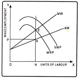
In the above fig MRP is the marginal revenue product curve and VMP is the value of marginal product curve. The VMP curve is above the MRP curve. The monopsonist is in equilibrium at point E. The monopsonist employs ON units of labour and wage rate OP is determined in the market.
Monopoly in the product market and monopsony in the factor market leads to the double exploitation of labour, i.e., monopolistic exploitation and monopsonist exploitation. At this equilibrium level monopolistic exploitation is EL while the monopsonist exploitation is equal to EK.
Key takeaways –
Meaning
David Ricardo defined rent as “that portion of the produce of the earth which is paid to the land lord for the use of original and indestructible powers of the soil”. Thus, rent is only a payment for the use of land. The following are the theories of rent: (i) Ricardian Theory of Rent, and (ii) Modern Theory of Rent.
Ricardian theory of rent
David Ricardo, an English classical economist, first developed a theory in 1817 to explain the origin and nature of economic rent. Ricardo used the economic and rent to analyse a particular question. In the Napoleonic wars (18.05-1815) there were large rise in corn and land prices.
He defined rent as “that portion of the produce of the earth which is paid to the landlord for the use of the original and indestructible powers of the soil.”
Assumption
Reasons for existence of rent
Let us assume that there are four types of land, classified based on its fertility, viz., A, B, C and D. A is the most fertile land and D is the least fertile land. People from the neighbouring place come in batches to settle on the land. The first batch of people will naturally cultivate the most fertile land, i.e., A grade land. Let us assume that one dose of labour and capital on ‘A’ quality land yields 20 quintals of paddy per acre. Then, the second batch of settlers has two alternatives - either to cultivate B quality land, which is free, or to take ‘A’ quality land on rent from the first batch. It is obvious that the rent payable on the ‘A’ quality land would be equal to the differences in the fertilities of A and B quality lands. Let us assume that one dose of labour and capital applied to ‘B’ quality land yields 18 quintals of paddy. Now the rent is equal to 2 quintals, i.e., 20-18 quintals of paddy, because this represents the difference between the fertilities of the two types of lands.
Return from different qualities of land | ||||
labour and capital | Returns (in quantils of paddy per acre) | |||
| A | B | C | D |
1 | 20 | 18 | 16 | 14 |
2 | 18 | 16 | 14 | 12 |
3 | 16 | 14 | 12 | 10 |
4 | 14 | 12 | 10 | 8 |
Even if the second batch decides not to take up A quality land on rent, rent would still arise on ‘A’ quality land. Since the market price of paddy will be equal to the cost of production at ‘B’ quality land, ‘A’ quality land will have a surplus over ‘B’ quality land. The surplus return for A quality land arises due to its superior fertility in comparison with the ‘B’ quality land. Suppose, if 10 doses of labour and capital are available, rent from various qualities of land will be:
Rent of A grade land = Total quantity of produce - Total cost
= 68 – 56 = 12 quintals
Rent of B grade = 48 - 42 = 6 quintals
Rent of C grade = 30 - 28 = 2 quintals
Rent of D grade = 14 - 14 = 0 (no rent)

In this example, D quality land is the marginal or no-rent land, because it earns no rent. Thus, rent arises on account of natural differential advantages of a piece of land over the marginal land. The natural differential advantages may be due to either superior quality of land or its better situation.
Criticisms of the Ricardian Theory of Rent
According to Ricardo, rent is due to the original and indestructible powers of the soil. But the fertility of the soil can be increased through manuring. Likewise, fertility of the soil can be destroyed through continuous cultivation without manuring.
In a thickly populated country, even the most inferior land yields rent and there is no marginal land in those countries. Thus, rent is not due to fertility, but to the scarcity of land.
Modern Theory of Rent
Economists like Alfred Marshall, Joan Robinson criticized Ricardian theory of Rent and put forward a new approach. They believed that rent does not arise due to fertility of the land rather it arises due to Scarcity of a factor. Although land is free gift of nature but it is not free for a firm or enterprise. They have to pay for its usage and the price is decided by the scarcity i.e. more scare the factor more price for it. So the availability of the factor affects its price. Here the concept of opportunity cost comes in play. Opportunity cost is the value of next best available alternative .A Factor needs to be paid minimum amount equal to its opportunity cost. Remember it is the minimum amount i.e. the lowest limit, actual amount may be much higher.
The actual amount to be paid depends on the scarcity and availability of that factor. If the factor is scare i.e. less available then the buyer has to pay more amount (Price) for that factor than its opportunity cost. This extra payment is nothing but Rent which depends on scarcity of a factor. Similarly for less scare factor buyer may pay an amount equal or slightly higher than its opportunity cost.
So rent is the extra payment over the opportunity cost (Minimum cost which has to be incurred). The scare factor attracts more rent as the difference in the opportunity cost and actual rent paid is more. Ricardo in his theory assumed that rent arises only on land but the advocates of Modern theory of rent believed that rent can arise on any factor of production.
Suppose an IT professional is working in firm A for a monthly package of Rs.one lakh. With the growing IT sector, the demand for IT professionals will increase. Now firm B offers him a monthly package of Rs. two lakh and he accepts the same.
Opportunity cost in above example = 1,00,000
Actual earning of factor = 2,00,000
Rent= Actual earning- Opportunity cost i.e. 200000-100000=100000
The rent of one lakh is result of scarcity of IT professionals i.e. demand of IT professionals are more than its supply as a result their price increases.
The scarcity of factor can be shown with the help of its Supply curve. If the factor is highly scare its supply curve will be vertical to the X axis or perfectly inelastic showing zero opportunity cost and whole amount as rent. On the other hand if the factor is not scare at all supply curve will be horizontal to the X axis or perfectly elastic one showing that the opportunity cost is equal to actual amount and hence Zero rent. So the shape of supply curve is the indicator of scarcity of the factor.

The above diagram shows the situation of no Rent. As you can see the supply cure is perfectly elastic indicating that the factor is not scare at all. Here the opportunity cost is same as the actual amount spent i.e. the minimum amount of opportunity cost is equal to the actual earning of the factor.

The above diagram shows the case of completely scare factor in which the whole earning is the amount of rent. Here the opportunity cost is zero and supply curve is perfectly inelastic. So whatever the demand for the factor determine its price and the whole amount represents the rent which is OPSE in the above diagram.
Quasi Rent
Quasi rent is the earning of capital equipments such as machineries, buildings etc., which are inelastic in supply, in short run. According to Marshall, the quasi rent is only a temporary surplus, which is enjoyed by the owner of the capital equipments in the short run. This is due to the increase in its demand and it will disappear in the long run, if supply of the capital equipment is increased in response to the increased demand. The quasi rent is also defined as the excess of total revenue earned in the short run over and above the total variable costs. Thus, Quasi Rent = Total Revenue Earned minus Total Variable Costs.
Ricardian rent is a payment made for the use of land whereas quasi-rent is a payment for man-made factors such as buildings, machineries, etc. Ricardian rent Wage Fund Rate of Wages = Number of Workers exists both in short run and long run because supply of land is fixed in long run. But quasi rent is only a temporary earning due to increased demand.
Key takeaways –
References


