Unit-4
Linear programming
We use linear programming to optimize the linear function subject to given linear constraints.
LPP is the popular mathematical technique which is used to make maximum profit and minimum loss.
Important definitions-
Linear programming problem-
We need to optimize the linear function Z subject to certain conditions, these types of problems are called Linear programming problem or in short LPP.
Objective functions-
This is a linear function of several variables, subject to the conditions.
Optimal value-
This is a maximum or minimum value of a object function which is to be calculated in a LPP.
Formulation of LPP-
Let’s consider the following example-
Example: A manufacturer produces two types of products ‘P’ and ‘Q’. Each ‘P’ type of product required 4 hours of grinding and 2 hrs of polishing, where ‘Q’ product requires 2 hrs of grinding and 5hrs of polishing.
The manufacturer has 2 grinders and 3 polishers. Each grinder works for 80hrs a week and each polisher works for 180hrs a week. Profit on ‘P’ product is Rs. 3 and profit on ‘Q’ is Rs. 4.Whatever is produced in a week is sold in the market.
How should the manufacturer allocate his capacity of production of two types of products so that he may make the maximum profit and minimum loss in a week?
Now we formulate this problem in mathematical terms as explained below-
Suppose  is the number of ‘P’ product and
  is the number of ‘Q’ product produced weekly.
Then the weekly profit is-

Here ‘Z’ is called the objective function which is to be maximize or minimize.
Now, to produce these number of products, the total number of grinding hours needed weekly is-

And the total number of polishing hours needed per week is-

Here the number of grinding hours is not more than 80 and the number of polishing hours is not more than 180, so that we write,
 This is called the first constraint]
 [This is the second constraint]
Since the number of product is non-negative, then we can write-

This is called the third constraint.
Hence we form the problem mathematically as follows-
To maximize- 
Subject to the constraints:


This expression is called as mathematical formulation.
Note- The variables that enter into the problem are called ‘decision variables’.
Example: A dietician mixes together two kinds of food, say, A and B in such a way that the mixture contains at least 6 units of vitamin P, 7 units of vitamin Q, 12 units of vitamin R and 9 units of vitamin S. The vitamin contents of 1 kg of food A and 1 kg of food B are given below:
Cost | Vitamin-P | Vitamin-Q | Vitamin-R | Vitamin-S |
Food-A | 1 | 1 | 1 | 2 |
Food-B | 2 | 1 | 3 | 1 |
One kg of food X costs Rs. 5, whereas one kg of food Y costs Rs. 8. Formulate the linear programming problem.
Sol.
Decision variables- Here decision variables are units of food A and B.
Let food A in the mixture be  and food B in the mixture
  .
.
Objective function- To minimize the cost,
Total cost of food A and B = 
Or

Now we will write the constraints one by one-
Constraint-1: 
Constraint-2: 
Constraint-3: 
Constraint-4: 
Constraint-5: 
Mathematical formation will be as follows-
To minimize,

Subject to the constraints-


Example: A manufacturer has 3 machines 1, 2 and 3. Machines 1 and 2 are capable of being operated for at the most 12 hours whereas machine 3 must be operated at least for 5 hours a day. He produces two items each requiring the use of the three machines.
The number of hours required for producing 1 unit of each of the items X and Y on the three machines are given below:
items | Numbers of hours required on the machines 1 2 3 |
X | 1 2 1 |
Y | 2 1 5/4 |
She makes a profit of Rs. 60 on item X and Rs. 40 on item Y. Assuming that he can sell all that he produces, how many of each item should be produced so as to maximize the profit. Formulate the above as L.P.P.
Sol-
Decision variables- Here decision variables are item X and Y.
Let the production of item X be  and the production of item Y be
  .
.
Objective function- To maximize the profit,

Now we will write the constraints one by one-
Constraint-1: 
Constraint-2: 
Constraint-3: 
Constraint-4: 
Mathematical formation will be as follows-
To maximize,

Subject to the constraints-


Key takeaways-
LPP having two variables can be easily solved by graphical method which provides a pictorial representation of the solution and we get insights into the basic concept used in solve LPP.
Step by step procedure to solve LPP graphically-

Note- The region satisfying all the constraints is called feasible region.
Example: Solve the following LPP graphically-
Maximize-

Subject to the constraints-


Sol.
Change the given constraints into equations-


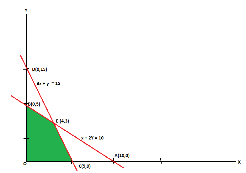
The line  meets the x-axis at the point A(10,0) and meets the y-axis at the point B(0,5). Join A and B to get the graph for the line.
Hence origin (0,0) satisfies the inequality  so that half plane containing the origin represent the solution set of
  .
.
And
The line  meets the x-axis at the point C(5,0) and meets the y-axis at the point D(0,15). Join C and D to get the graph for the line.
Hence origin (0,0) satisfies the inequality so that half plane containing the origin represent the solution set of
 .
.
Now all the points in first quadrant satisfies  .
.
So that first quadrant is the region represented by 
Hence the region OCEBO satisfies all the inequalities.
And each point on the region is the feasible solution of the problem.
Feasible solution-
Here in this problem the feasible solution is (5,0), (4,3) and (0,5).
Now we can obtain the optimal solution of the problem.
As we know that any point in the feasible region that gives the optimal value is called an optimal solution.

The value of the objective function  at corner points of the feasible region is given below-
vertex [ feasible region ] | Value of |
O(0,0) | 0 |
C(5,0) | 15 |
E(4,3) | 18 [Maximum] |
B(0,5) | 10 |
Here we see that the maximum value of Z is 18.

Note-
Example: Find the maximum value of Z = 2x + 3y subject to the constraints-

Sol.
Any point (x,y) satisfying the conditions  lies in the first quadrant only.
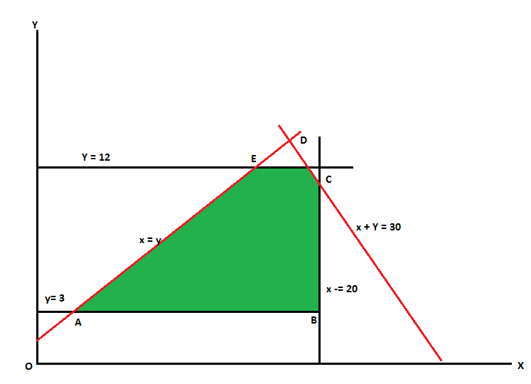
Also since  the desired point (x,y) lies within the convex region ABCDE.
Its vertices are A(3,3), B(20,3), C(20,10), D(18,12) and E(12,12).

The value of Z at these points are-
Z(A) = 15
Z(B) = 49
Z(C) = 70
Z(D) = 72
Z(E) = 60
Here 72 is the maximum value which is at D.
So that the solution of the LPP is x = 18 and y = 12 and maximum Z = 72
Example: A factory manufactures two types of items, A and B, each type requiring the use of two machines, an automatic and a hand operated. It takes 4 minutes on the automatic and 6 minutes on hand operated machines to manufacture a package of item A, while it takes 6 minutes on automatic and 3 minutes on the hand operated machines to manufacture a package of item B. Each machine is available for at the most 4 hours on any day. The manufacturer can sell a package of item A at a profit of Rs. 7 and item B at a profit of Rs 10. Assuming that he can sell all the items he manufactures, how many packages of each type should the factory owner produce in a day in order to maximise his profit ?
Determine the maximum profit.
Sol.
We can tabulate the data as follows-
Items \ Machine | Automatic operated | By hand operated | profit |
A | 4 min | 6 min | Rs. 7 |
B | 6 min | 3 min | Rs. 10 |
| 4 hours or[240 min] | 4 hours or[240 min] |
|
Decision variables- Let the manufacturer produce x packages of item A and y packages of item B per day respectively.
Objective function- Suppose Z denotes the maximum profit,

Constraints-
1st constraint-

2nd constraint-

3rd constraint-

Mathematical formulation-
The mathematical form of this LPP can be written as-
Maximize
Subject to the constraints-


Tables for the region represented by inequalities-
For the first constraint-

x | 60 | 0 |
y | 0 | 40 |
points | A | B |
For second condition- 
x | 40 | 0 |
y | 0 | 80 |
points | C | D |
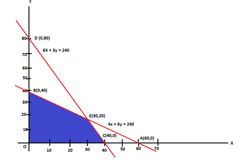
Now we draw on x and y axes.

The coordinates of the vertices O, C, E and B of the feasible region OCEBO are O (0, 0), C (40, 0), E (30, 20) and B (0, 40). The coordinates of E are obtained by solving the equations 4x + 6y = 240 and 6x + 3y = 240.
Corner points of the feasible region | Value of Z = 7x + 10y |
C (40, 0) | 280 |
E(30,20) | 410 [Maximum] |
B(0, 40) | 400 |
Therefore Z is maximum at x = 30 and y = 20 and the maximum value of Z is 410.
References-
