UNIT 3
Correlation
Correlation is used to describe the linear relationship between two continuous variables (e.g., height and weight). In general, correlation tends to be used when there is no identified response variable. It measures the strength (qualitatively) and direction of the linear relationship between two or more variables.
Definition
“Correlation analysis deals with the association between two or more variables.” —Simpson and Kafka
“Correlation is an analysis of the co-variation between two variables.” —A.M. Tuttle
Uses and types
Uses-
3. Validity: A test’s width value can be obtained through correlation. Whenever a test is constructed the tests, not what it claims to test.
4. Test Construction: The coefficient of correlation is also being used in the test construction. There are always the questions whenever a new test is constructed, whether each element of the test is related to other elements or to the test as a whole and as to whether each element is related to the criteria chosen. Those relationships are all examined through the technique of correlation.
Types
Correlation measures the nature and strength of relationship between two variables. Correlation lies between +1 to -1. A correlation of +1 indicates a perfect positive correlation between two variables. A zero correlation indicates that there is no relationship between the variables. A correlation of -1 indicates a perfect negative correlation.
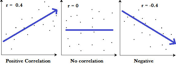
Degree of Correlation and its Nature
a) Coefficient of correlation (r) = 1: If there is perfect positive relationship between two variables, then the value of correlation will be +1.
b) Coefficient of correlation (r) = −1: If there is perfect negative relationship between two variables, then the value of correlation will be −1.
2. Zero correlation: The correlation is zero is said to be when two variables have no relationship between them. It implies that a change in the value of one variable has no effect on the change in the value of the other variable.
a) Coefficient of correlation (r) = 0: If there is no relationship between the two variables, then the value of correlation will be zero. However, it does not imply that these two variables are independent. It only indicates non-existence of linear relation between the two variables.
3. Limited degree of correlation: A limited degree of correlation exists between perfect correlation and zero correlation, i.e. the value of the coefficient of correlation lies between +1 and −1. This limited degree of correlation may be high, moderate or low.
a) High degree of correlation: Correlation of two series of data is closer to one.
b) Medium degree of correlation: Correlation of two series of data is neither large nor small.
c) Low degree of correlation: Correlation of two series of data is small.
Key takeaways –
Karl Pearson’s Coefficient of Correlation
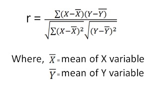
It is widely used mathematical method is used to calculate the degree and direction of the relationship between linear related variables. The coefficient of correlation is denoted by “r”.
Direct method-
Shortcut method –


The value of the coefficient of correlation (r) always lies between ±1. Such as:
a) r=+1, perfect positive correlation.
b) r=-1, perfect negative correlation.
c) r=0, no correlation.
Example 1 - Compute Pearsons coefficient of correlation between advertisement cost and sales as per the data given below:
Advertisement cost | 39 | 65 | 62 | 90 | 82 | 75 | 25 | 98 | 36 | 78 |
sales | 47 | 53 | 58 | 86 | 62 | 68 | 60 | 91 | 51 | 84 |
Solution
X | Y |
|
|
|
| |
39 | 47 | -26 | 676 | -19 | 361 | 494 |
65 | 53 | 0 | 0 | -13 | 169 | 0 |
62 | 58 | -3 | 9 | -8 | 64 | 24 |
90 | 86 | 25 | 625 | 20 | 400 | 500 |
82 | 62 | 17 | 289 | -4 | 16 | -68 |
75 | 68 | 10 | 100 | 2 | 4 | 20 |
25 | 60 | -40 | 1600 | -6 | 36 | 240 |
98 | 91 | 33 | 1089 | 25 | 625 | 825 |
36 | 51 | -29 | 841 | -15 | 225 | 435 |
78 | 84 | 13 | 169 | 18 | 324 | 234 |
650 | 660 |
| 5398 |
| 2224 | 2704 |
|
|
|
|
|
|
|

r = (2704)/√5398 √2224 = (2704)/(73.2*47.15) = 0.78
Thus Correlation coefficient is positively correlated
Example 2
Compute correlation coefficient from the following data
Hours of sleep (X) | Test scores (Y) |
8 | 81 |
8 | 80 |
6 | 75 |
5 | 65 |
7 | 91 |
6 | 80 |
X | Y |
|
|
|
| |
8 | 81 | 1.3 | 1.8 | 2.3 | 5.4 | 3.1 |
8 | 80 | 1.3 | 1.8 | 1.3 | 1.8 | 1.8 |
6 | 75 | -0.7 | 0.4 | -3.7 | 13.4 | 2.4 |
5 | 65 | -1.7 | 2.8 | -13.7 | 186.8 | 22.8 |
7 | 91 | 0.3 | 0.1 | 12.3 | 152.1 | 4.1 |
6 | 80 | -0.7 | 0.4 | 1.3 | 1.8 | -0.9 |
40 | 472 |
| 7 |
| 361 | 33 |

X = 40/6 =6.7

Y = 472/6 = 78.7

r = (33)/√7 √361 = (33)/(2.64*19) = 0.66
Thus Correlation coefficient is positively correlated
Example 3
Calculate coefficient of correlation between X and Y series using Karl pearson shortcut method
X | 14 | 12 | 14 | 16 | 16 | 17 | 16 | 15 |
Y | 13 | 11 | 10 | 15 | 15 | 9 | 14 | 17 |
Solution
Let assumed mean for X = 15, assumed mean for Y = 14
X | Y | dx | dx2 | dy | dy2 | dxdy |
14 | 13 | -1.0 | 1.0 | -1.0 | 1.0 | 1.0 |
12 | 11 | -3.0 | 9.0 | -3.0 | 9.0 | 9.0 |
14 | 10 | -1.0 | 1.0 | -4.0 | 16.0 | 4.0 |
16 | 15 | 1.0 | 1.0 | 1.0 | 1.0 | 1.0 |
16 | 15 | 1.0 | 1.0 | 1.0 | 1.0 | 1.0 |
17 | 9 | 2.0 | 4.0 | -5.0 | 25.0 | -10.0 |
16 | 14 | 1 | 1 | 0 | 0 | 0 |
15 | 17 | 0 | 0 | 3 | 9 | 0 |
120 | 104 | 0 | 18 | -8 | 62 | 6 |

 r = 8 *6 – (0)*(-8)
√8*18-(0)2 √8*62 – (-8)2
r = 48/√144*√432 = 0.19
Example 4 –
Calculate coefficient of correlation between X and Y series using Karl pearson shortcut method
X | 1800 | 1900 | 2000 | 2100 | 2200 | 2300 | 2400 | 2500 | 2600 |
F | 5 | 5 | 6 | 9 | 7 | 8 | 6 | 8 | 9 |
Solution
Assumed mean of X and Y is 2200, 6
X | Y | dx | dx (i=100) | dx2 | dy | dy2 | dxdy |
1800 | 5 | -400 | -4 | 16 | -1.0 | 1.0 | 4.0 |
1900 | 5 | -300 | -3 | 9 | -1.0 | 1.0 | 3.0 |
2000 | 6 | -200 | -2 | 4 | 0.0 | 0.0 | 0.0 |
2100 | 9 | -100 | -1 | 1 | 3.0 | 9.0 | -3.0 |
2200 | 7 | 0 | 0 | 0 | 1.0 | 1.0 | 0.0 |
2300 | 8 | 100 | 1 | 1 | 2.0 | 4.0 | 2.0 |
2400 | 6 | 200 | 2 | 4 | 0 | 0 | 0.0 |
2500 | 8 | 300 | 3 | 9 | 2 | 4 | 6.0 |
2600 | 9 | 400 | 4 | 16 | 3 | 9 | 12.0 |
|
|
|
|
|
|
|
|
|
|
| 0 | 60 | 9 | 29 | 24 |
Note – we can also proceed dividing x/100
 r = (9)(24) – (0)(9)
√9*60-(0)2 √9*29– (9)2
r = 0.69
Example 5 –
X | 28 | 45 | 40 | 38 | 35 | 33 | 40 | 32 | 36 | 33 |
Y | 23 | 34 | 33 | 34 | 30 | 26 | 28 | 31 | 36 | 35 |
Solution
X | Y |
|
|
|
| |
28 | 23 | -8 | 64 | -8.0 | 64.0 | 64.0 |
45 | 34 | 9 | 81 | 3.0 | 9.0 | 27.0 |
40 | 33 | 4 | 16 | 2.0 | 4.0 | 8.0 |
38 | 34 | 2 | 4 | 3.0 | 9.0 | 6.0 |
35 | 30 | -1 | 1 | -1.0 | 1.0 | 1.0 |
33 | 26 | -3 | 9 | -5.0 | 25.0 | 15.0 |
40 | 28 | 4 | 16 | -3 | 9 | -12.0 |
32 | 31 | -4 | 16 | 0 | 0 | 0.0 |
36 | 36 | 0 | 0 | 5 | 25 | 0.0 |
33 | 35 | -3 | 9 | 4 | 16 | -12 |
360 | 310 | 0 | 216 | 0 | 162 | 97 |

 X = 360/10 = 36
Y = 310/10 = 31

r = 97/(√216 √162 = 0.51
Spearman’s Rank Correlation Coefficient –
The Spearman’s Rank Correlation Coefficient is the non-parametric statistical measure used to study the strength of association between the two ranked variables. This method is used for ordinal set of numbers, which can be arranged in order.

Where, P = Rank coefficient of correlation
D = Difference of ranks
N = Number of Observations
The Spearman’s Rank Correlation coefficient lies between +1 to -1.
d) +1 indicates perfect association of rank
e) 0 indicates no association between the rank
f) -1 indicates perfect negative association between the ranks
When ranks are not given - Rank by taking the highest value or the lowest value as 1
Equal Ranks or Tie in Ranks – in this case ranks are assigned on an average basis. For ex – if three students score of 5, at 5th, 6th, 7th ranks ach one of them will be assigned a rank of 5 + 6 + 7/3= 6.
If two individual ranked equal at third position, then the rank is calculates as (3+4)/2 = 3.5
Example 1 –
Test 1 | 8 | 7 | 9 | 5 | 1 |
Test 2 | 10 | 8 | 7 | 4 | 5 |
Solution
Here, highest value is taken as 1
Test 1 | Test 2 | Rank T1 | Rank T2 | d | d2 |
8 | 10 | 2 | 1 | 1 | 1 |
7 | 8 | 3 | 2 | 1 | 1 |
9 | 7 | 1 | 3 | -2 | 4 |
5 | 4 | 4 | 5 | -1 | 1 |
1 | 5 | 5 | 4 | 1 | 1 |
|
|
|
|
| 8 |

R = 1 – (6*8)/5(52 – 1) = 0.60
Example 2 -
Calculate Spearman rank-order correlation
English | 56 | 75 | 45 | 71 | 62 | 64 | 58 | 80 | 76 | 61 |
Maths | 66 | 70 | 40 | 60 | 65 | 56 | 59 | 77 | 67 | 63 |
Solution
Rank by taking the highest value or the lowest value as 1.
Here, highest value is taken as 1
English | Maths | Rank (English) | Rank (Math) | d | d2 |
56 | 66 | 9 | 4 | 5 | 25 |
75 | 70 | 3 | 2 | 1 | 1 |
45 | 40 | 10 | 10 | 0 | 0 |
71 | 60 | 4 | 7 | -3 | 9 |
62 | 65 | 6 | 5 | 1 | 1 |
64 | 56 | 5 | 9 | -4 | 16 |
58 | 59 | 8 | 8 | 0 | 0 |
80 | 77 | 1 | 1 | 0 | 0 |
76 | 67 | 2 | 3 | -1 | 1 |
61 | 63 | 7 | 6 | 1 | 1 |
|
|
|
|
| 54 |

 R = 1-(6*54)
10(102-1)
R = 0.67
There fore this indicates a strong positive relationship between the ranks individuals obtained in the math and English exam.
Example 3 –
Find Spearman's rank correlation coefficient between X and Y for this set of data:
X | 13 | 20 | 22 | 18 | 19 | 11 | 10 | 15 |
Y | 17 | 19 | 23 | 16 | 20 | 10 | 11 | 18 |
Solution
X | Y | Rank X | Rank Y | d | d2 |
13 | 17 | 3 | 4 | -1 | 1 |
20 | 19 | 7 | 6 | 1 | 1 |
22 | 23 | 8 | 8 | 0 | 0 |
18 | 16 | 5 | 3 | 2 | 2 |
19 | 20 | 6 | 7 | -1 | 1 |
11 | 10 | 2 | 1 | 1 | 1 |
10 | 11 | 1 | 2 | -1 | 1 |
15 | 18 | 4 | 5 | -1 | 1 |
|
|
|
|
| 8 |
R =

 R = 1 – 6*8/8(82 – 1) = 1 – 48 = 0.90
504
Example 4 – Calculation of equal ranks or tie ranks
Find Spearman's rank correlation coefficient:
Commerce | 15 | 20 | 28 | 12 | 40 | 60 | 20 | 80 |
Science | 40 | 30 | 50 | 30 | 20 | 10 | 30 | 60 |
Solution
C | S | Rank C | Rank S | d | d2 |
15 | 40 | 2 | 6 | -4 | 16 |
20 | 30 | 3.5 | 4 | -0.5 | 0.25 |
28 | 50 | 5 | 7 | -2 | 4 |
12 | 30 | 1 | 4 | -3 | 9 |
40 | 20 | 6 | 2 | 4 | 16 |
60 | 10 | 7 | 1 | 6 | 36 |
20 | 30 | 3.5 | 4 | -0.5 | 0.25 |
80 | 60 | 8 | 8 | 0 | 0 |
|
|
|
|
| 81.5 |

R = 1 – (6*81.5)/8(82 – 1) = 0.02
Example 5 –
X | 10 | 15 | 11 | 14 | 16 | 20 | 10 | 8 | 7 | 9 |
Y | 16 | 16 | 24 | 18 | 22 | 24 | 14 | 10 | 12 | 14 |
Solution
X | Y | Rank X | Rank Y | d | d2 |
10 | 16 | 6.5 | 5.5 | 1 | 1 |
15 | 16 | 3 | 5.5 | -2.5 | 6.25 |
11 | 24 | 5 | 1.5 | 3.5 | 12.25 |
14 | 18 | 4 | 4 | 0 | 0 |
16 | 22 | 2 | 3 | -1 | 1 |
20 | 24 | 1 | 1.5 | -0.5 | 0.25 |
10 | 14 | 6.5 | 7.5 | -1 | 1 |
8 | 10 | 9 | 10 | -1 | 1 |
7 | 12 | 10 | 9 | 1 | 1 |
9 | 14 | 8 | 7.5 | 0.5 | 0.25 |
|
|
|
|
| 24 |

R = 1 – (6*24)/10(102 – 1) = 0.85
The correlation between X and Y is positive and very high.
Key takeaways - Correlation is used to describe the linear relationship between two continuous variables
Regression analysis is a technique of studying the dependence of one variable called dependent variable, on one or more variable called explanatory variable, with a view to estimate or predict the average value of the dependent variables in terms of the known or fixed values of the independent variables.
Regression analysis includes several variations, such as linear, multiple linear, and nonlinear. The most common models are simple linear and multiple linear.
Nonlinear regression analysis is commonly used for more complicated data sets in which the dependent and independent variables show a nonlinear relationship.
Linear model assumption -
Importance
Regression Analysis, a statistical technique, is used to evaluate the relationship between two or more variables. Regression analysis helps an organisation to understand what their data points represent and use them accordingly with the help of business analytical techniques in order to do better decision-making. In this analysis, you will understand how the typical value of the dependent variable changes when one of the independent variables is varied, while the other independent variables are held fixed. Business analysts and data professionals use this powerful statistical tool for removing the unwanted variables and select the important ones.
Simple linear regression
Simple linear regression is a model that assesses the relationship between a dependent variable and an independent variable.
Y = a + bX + ϵ
Where:
Y – Dependent variable
X – Independent (explanatory) variable
a – Intercept
b – Slope
ϵ – Residual (error)
With the help of simple linear regression model we have the following two regression lines
1. Regression line of Y on X: This line gives the probable value of Y (Dependent variable) for any given value of X (Independent variable).
Regression line of Y on X : Y – Ẏ = byx (X – Ẋ)
OR : Y = a + bX
2. Regression line of X on Y: This line gives the probable value of X (Dependent variable) for any given value of Y (Independent variable).
Regression line of X on Y : X – Ẋ = bxy (Y – Ẏ)
OR : X = a + bY
Multiple linear regressions-
Multiple linear regression analysis is essentially similar to the simple linear model, with the exception that multiple independent variables are used in the model.
Y = a + bX1 + cX2 + dX3 + ϵ
Where:
Y – Dependent variable
X1, X2, X3 – Independent (explanatory) variables
a – Intercept
b, c, d – Slopes
ϵ – Residual (error)
Example
How to find a linear regression equation
Subject | X | Y |
1 | 43 | 99 |
2 | 21 | 65 |
3 | 25 | 79 |
4 | 42 | 75 |
5 | 57 | 87 |
6 | 59 | 81 |
|
|
|
Solution
Subject | X | Y | Xy | X2 | Y2 |
1 | 43 | 99 | 4257 | 1849 | 9801 |
2 | 21 | 65 | 1365 | 441 | 4225 |
3 | 25 | 79 | 1975 | 625 | 6241 |
4 | 42 | 75 | 3150 | 1764 | 5625 |
5 | 57 | 87 | 4959 | 3249 | 7569 |
6 | 59 | 81 | 4779 | 3481 | 6521 |
Total | 247 | 486 | 20485 | 11409 | 40022 |
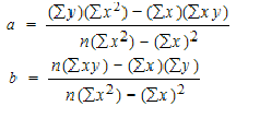
To find a and b, use the following equation
Find a:
((486 × 11,409) – ((247 × 20,485)) / 6 (11,409) – 247*247)
484979 / 7445
=65.14
Find b:
(6(20,485) – (247 × 486)) / (6 (11409) – 247*247)
(122,910 – 120,042) / 68,454 – 2472
2,868 / 7,445
= .385225
y’ = a + bx
y’ = 65.14 + .385225x
Example
Calculate linear regression analysis
students | X | Y |
1 | 95 | 85 |
2 | 85 | 95 |
3 | 80 | 70 |
4 | 70 | 65 |
5 | 60 | 70 |
Solution
students | X | Y | X2 | y2 | xy |
1 | 95 | 85 | 9025 | 7225 | 8075 |
2 | 85 | 95 | 7225 | 9025 | 8075 |
3 | 80 | 70 | 6400 | 4900 | 5600 |
4 | 70 | 65 | 4900 | 4225 | 4550 |
5 | 60 | 70 | 3600 | 4900 | 4200 |
total | 390 | 385 | 31150 | 30275 | 30500 |
To find a and b, use the following equation
Find a:
((385 × 31150) – ((390 × 30500)) / 5 (31150) – 152100)
97750 / 3650
=26.78
Find b:
(5(30500) – (390 × 385)) / (5 (31150) – 152100)
2,350 / 3650
= .0.64
y’ = a + bx
y’ = 26.78 + .0.64x
Key takeaways - Regression analysis includes several variations, such as linear, multiple linear, and nonlinear. The most common models are simple linear and multiple linear
The standard error is one of the mathematical tools used in statistics to estimate the variability. It is abbreviated as SE. The standard error of a statistic or an estimate of a parameter is the standard deviation of its sampling distribution. We can define it as an estimate of that standard deviation.
The accuracy of a sample that describes a population is identified through SE formula. The sample mean which deviates from the given population and that deviation is given as;


Where S is the standard deviation and n is the number of observations.
The standard error of the estimate is the estimation of the accuracy of any predictions. It is denoted as SEE. The regression line depreciates the sum of squared deviations of prediction. It is also known as the sum of squares error. SEE is the square root of the average squared deviation. The deviation of some estimate from intended values is given by standard error of estimate formula.

How to calculate Standard Error
Step 1: Note the number of measurements (n) and determine the sample mean (μ). It is the average of all the measurements.
Step 2: Determine how much each measurement varies from the mean.
Step 3: Square all the deviations determined in step 2 and add altogether: Σ(xi – μ)²
Step 4: Divide the sum from step 3 by one less than the total number of measurements (n-1).
Step 5: Take the square root of the obtained number, which is the standard deviation (σ).
Step 6: Finally, divide the standard deviation obtained by the square root of the number of measurements (n) to get the standard error of your estimate.
Calculate the standard error of the given data:
y: 5, 10, 12, 15, 20
Solution: First we have to find the mean of the given data;
Mean = (5+10+12+15+20)/5 = 62/5 = 10.5
Now, the standard deviation can be calculated as;
S = Summation of difference between each value of given data and the mean value/Number of values.
Hence,
After solving the above equation, we get;
S = 5.35
Therefore, SE can be estimated with the formula;
SE = S/√n
SE = 5.35/√5 = 2.39
Key takeaways - The standard error of the estimate is the estimation of the accuracy of any predictions. It is denoted as SEE.
The value of money does not remain same over the time. A rise in the price levels means a fall in the value of money and a fall in the price level means a rise in the value of money. Thus index number is a statistical device that measures the relative change in the level of price from one time period to another.
Definition
“Index numbers are quantitative measures of growth of prices, production, inventory and other quantities of economic interest” ………Ronold
An index number measures how much a variable changes over the time. Index number is calculated by finding the ratio of current value to a base value.
Uses of index number
a) Index numbers are specialized averages.
b) Index numbers measures the change in one variable or a group of variables.
c) Index numbers measures the effect of changes over a period of time.
d) Index numbers are meant to study the changes in the effects of such factors which cannot be measured directly.
Types of index number
1. Wholesale Price Index Numbers:
Wholesale price index numbers are constructed on the basis of the wholesale prices of certain important commodities. The commodities included in preparing these index numbers are mainly raw-materials and semi-finished goods. Only the most important and most price-sensitive and semi- finished goods which are bought and sold in the wholesale market are selected and weights are assigned in accordance with their relative importance.
2. Retail Price Index Numbers:
These index numbers are prepared to measure the changes.in the value of money on the basis of the retail prices of final consumption goods. The main difficulty with this index number is that the retail price for the same goods and for continuous periods is not available. The retail prices represent larger and more frequent fluctuations as compared to the wholesale prices.
3. Cost-of-Living Index Numbers:
These index numbers are constructed with reference to the important goods and services which are consumed by common people. Since the number of these goods and services is very large, only representative items which form the consumption pattern of the people are included. These index numbers are used to measure changes in the cost of living of the general public.
4. Working Class Cost-of-Living Index Numbers:
The working class cost-of-living index numbers aim at measuring changes in the cost of living of workers. These index numbers are consumed on the basis of only those goods and services which are generally consumed by the working class. The prices of these goods and index numbers are of great importance to the workers because their wages are adjusted according to these indices.
5. Wage Index Numbers:
The purpose of these index numbers is to measure time to time changes in money wages. These index numbers, when compared with the working class cost-of-living index numbers, provide information regarding the changes in the real wages of the workers.
6. Industrial Index Numbers:
Industrial index numbers are constructed with an objective of measuring changes in the industrial production. The production data of various industries are included in preparing these index numbers.
Methods of constructing price index number, fixed base method, chain base method, fishers’s ideal index number
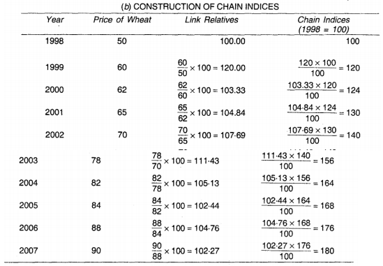
The chain index numbers - In fixed base method the base remain constant through out i.e. the relatives for all the years are based on the price of that single year. On the other hand in chain base method, the relatives for each year is found from the prices of the immediately preceding year. Thus the base changes from year to year. Such index numbers are useful in comparing current year figures with the preceding year figures. The relatives which we found by this method are called link relatives.
Thus link relative for current year = current years figure/previous year figure *100
And by using these link relatives we can find the chain indices for each year by using the below formula
Chain index for current year = Link relative of current year * Chain index of previous year/ 100
Note: The fixed base index number computed from the original data and chain index number computed from link relatives give the same value of the index provided that there is only one commodity, whose indices are being constructed.
Example 1
From the following data of wholesale prices of wheat for ten years construct index number taking a) 1998 as base and b) by chain base method


Example 2
From the following data calculate the index numbers using the Chain Index Numbers method.
Year 2011 2012 2013 2014 2015 2016 2017 2018
Prices 120 124 130 144 150 160 164 170
Solution
Construction of Chain Index Numbers
Year | Price | Link Relatives | Chain indices |
2011 | 120 | 100 | 100 |
2012 | 124 | 120/124 x 100 = 103.33 | 103.33 ×100/100 = 103.33 |
2013 | 130 | 124/130 x 100 = 104.83 | 104.83 ×103.33/100 = 108.32 |
2014 | 144 | 130/144 x 100 = 110.76 | 110.76×108.32 /100= 119.98 |
2015 | 150 | 144/150 x 100 = 104.16 | 104.16 ×119.98/100 = 124.97 |
2016 | 160 | 150/160 x 100 = 106.66 | 106.66×124.97/100 = 133.29 |
2017 | 164 | 160/164 x 100 = 102.5 | 102.5 ×133.29/100 = 136.62 |
2018 | 170 | 164/170 x 100 = 103.65 | 103.65 ×136.62/100 = 141.61 |
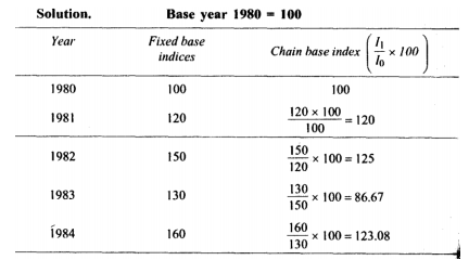
Example 3
Compute the chain base index numbers
Solution

Fixed base method – under this method index number is calculated with a fixed base year. By this method the index number of a given year is not influenced by the variation of prices of any other year.
Price relatrive of current year = price of current year/ price of base year*100
Example 1
Find index numbers for the following data taking 1980 as the base year.
Year | 1980 | 1981 | 1982 | 1983 | 1984 | 1985 | 1986 | 1987 |
Price | 40 | 50 | 60 | 70 | 80 | 100 | 90 | 110 |
Solution

Construction of price index numbers

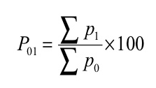
Where, P01 = Index number
P 1= Total of the current year’s prices of all commodities
P 0= Total of the base year’s prices of all commodities
Examples 1–
Commodity | Price in base year 2005 | Price in current year 2010 |
A | 10 | 20 |
B | 15 | 25 |
C | 40 | 60 |
D | 25 | 40 |
Solution
Commodity | Price in base year 2005 | Price in current year 2010 |
A | 10 | 20 |
B | 15 | 25 |
C | 40 | 60 |
D | 25 | 40 |
|
|
|
Index number ( P01 ) = 
P01 = (145/90)*100 = 161.11
It means the price in 2010 were 61% more than the price in 2005
Example 2
Find the index number from the data given below
Commodities | Units | Price in 2007 | Price in 2008 |
Sugar | Quintal | 2200 | 3200 |
Milk | Quintal | 18 | 20 |
Oil | Liter | 68 | 71 |
Wheat | Quintal | 900 | 1000 |
Clothing | Meter | 50 | 60 |
|
|
|
|
Solution
Commodities | Units | Price in 2007 | Price in 2008 |
Sugar | Quintal | 2200 | 3200 |
Milk | Quintal | 18 | 20 |
Oil | Liter | 68 | 71 |
Wheat | Quintal | 900 | 1000 |
Clothing | Meter | 50 | 60 |
|
|
|
|
Index number ( P01 ) = 
P01 = (4351/3236)*100 = 134.45
It means the price in 2008 were 34% more than the price in 2007
Example 3 –
Construct the price index for 2003, taking the year 2000 as base year
Commodities | Price in 2000 | Price in 2003 |
A | 60 | 80 |
B | 50 | 60 |
C | 70 | 100 |
D | 120 | 160 |
E | 100 | 150 |
|
|
|
Solution
Commodities | Price in 2000 - P 0 | Price in 2003 - P 1 |
A | 60 | 80 |
B | 50 | 60 |
C | 70 | 100 |
D | 120 | 160 |
E | 100 | 150 |
|
|
|
Index number ( P01 ) = 
P01 = (550/400)*100 = 137.5
Therefore there is an increase of 37.5% in the prices in 2003 as against 2000.
Example 4-
Compute the price index for the years 2001, 2002, 2003, 2004 taking 2000 as base year
Year | 2000 | 2001 | 2002 | 2003 | 2004 |
Price | 120 | 144 | 168 | 204 | 216 |
Solution
Price index for different years
2000 | (120/120)*100 = 100 |
2001 | (144/120)*100 = 120 |
2002 | (168/120)*100 = 140 |
2003 | (204/120)*100 = 170 |
2004 | (216/120)*100 = 180 |
Example 5 –
Prepare simple aggregative price index
Commodities | Price in 1995 - P 0 | Price in 2003 - P 1 |
Wheat | 100 | 140 |
Rice | 200 | 250 |
Pulses | 250 | 350 |
Sugar | 14 | 20 |
Oil | 40 | 50 |
Solution
Commodities | Price in 1995 - P 0 | Price in 2003 - P 1 |
Wheat | 100 | 140 |
Rice | 200 | 250 |
Pulses | 250 | 350 |
Sugar | 14 | 20 |
Oil | 40 | 50 |
|
|
|
Simple aggregative index number = (810/604)*100 = 134.1
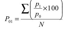
2. Simple average of relative method - in this method, index number is equal to the sum of price relatives divided by the number of items.

Where, N= number of items
Example 1 –
Commodity | Base year | Current year |
A | 10 | 20 |
B | 15 | 25 |
C | 40 | 60 |
D | 25 | 40 |
|
|
|
Solution
Commodity | Base year | Current year | Price relatives |
A | 10 | 20 | (20/10)*100 = 200 |
B | 15 | 25 | (25/15)*100 =166.7 |
C | 40 | 60 | (60/40)*100 =150 |
D | 25 | 40 | (40/25)*100 =160 |
N = 4 |
|
|
|

Index number = 676.7/4 = 169.2
Example 2 –
Construct the index number for the year 2010
Commodities | Price (2009) | Price(2010) |
P | 6 | 10 |
Q | 12 | 2 |
R | 4 | 6 |
S | 10 | 12 |
T | 8 | 12 |
|
|
|
Solution
Commodities | Price (2009) | Price(2010) | Price relative |
P | 6 | 10 | 166.67 |
Q | 12 | 2 | 16.67 |
R | 4 | 6 | 150 |
S | 10 | 12 | 120 |
T | 8 | 12 | 150 |
N = 5 |
|
| 603.34 |

Index number = 603.34/4 = 120.68
Example 3 –
Using simple average of price relative method find price index for 2001, taking 1996 as base year for the following data
Commodity | Wheat | Rice | Sugar | Ghee | Tea |
Price in 1996 | 12 | 20 | 12 | 40 | 80 |
Price in 2001 | 16 | 25 | 16 | 60 | 96 |
Solution
Commodities | Price (2009) | Price(2010) | Price relative |
Wheat | 12 | 16 | (16/12)*100 = 133.33 |
Rice | 20 | 25 | (25/20)*100 = 125 |
Sugar | 12 | 16 | 133.33 |
Ghee | 40 | 60 | 150 |
Tea | 80 | 96 | 120 |
N = 5 |
|
| 661.66 |

 =661.66 = 132.33
5
Therefore Price Index for 2001, taking 1996 as base year, = 132.33
Example 4 –
Using simple average of price relative method find price index for 2010, taking 2009 as base year for the following data
Commodities | Price (2009) | Price(2010) |
A | 60 | 80 |
B | 50 | 60 |
C | 60 | 72 |
D | 50 | 75 |
E | 25 | 37 .5 |
F | 20 | 30 |
Solution
Commodities | Price (2009) | Price(2010) | Price relatives |
A | 60 | 80 | 133.33 |
B | 50 | 60 | 120 |
C | 60 | 72 | 120 |
D | 50 | 75 | 150 |
E | 25 | 37 .5 | 150 |
F | 20 | 30 | 150 |
N = 6 |
|
| 823.33 |

= 823.33/6 = 137.22
3. Weighted aggregative method – in this method, according to the relative importance, different weights are assigned to the items. Many formulas developed to estimate index numbers on the basis of weights.
Some of the formulas given below


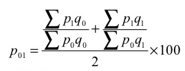


Where q refers to quantity of some period, not necessarily of the mean of the base year and current year.
Example 1 –
Commodity | Base year | Current year | ||
PO | QO | P1 | Q1 | |
A | 10 | 5 | 20 | 2 |
B | 15 | 4 | 25 | 8 |
C | 40 | 2 | 60 | 6 |
D | 25 | 3 | 40 | 4 |
Solution
Commodity | Base year | Current year |
|
|
|
| ||
PO | QO | P1 | Q1 | Poqo | P1qo | Poq1 | P1q1 | |
A | 10 | 5 | 20 | 2 | 50 | 100 | 20 | 40 |
B | 15 | 4 | 25 | 8 | 60 | 100 | 120 | 200 |
C | 40 | 2 | 60 | 6 | 80 | 120 | 240 | 360 |
D | 25 | 3 | 40 | 4 | 75 | 120 | 100 | 160 |
|
|
|
|
| 265 | 440 | 480 | 760 |
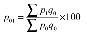
P 01 = (440/265)*100 = 166.04

P 01 = (760/480)*100 = 158.33

 P 01 = ((440/265) + (760/480)) *100 = 162
2

 P 01 = √ ((440/265) + (760/480)) *100 = 162.1
Example 2
Commodity | Base year | Current year | ||
PO | QO | P1 | Q1 | |
A | 15 | 500 | 20 | 600 |
B | 18 | 590 | 23 | 640 |
C | 22 | 450 | 24 | 500 |
Solution
Commodity | Base year | Current year |
|
|
|
| ||
PO | QO | P1 | Q1 | Poqo | P1qo | Poq1 | P1q1 | |
A | 15 | 500 | 20 | 600 | 7500 | 10000 | 9000 | 12000 |
B | 18 | 590 | 23 | 640 | 10620 | 13570 | 11520 | 14720 |
C | 22 | 450 | 24 | 500 | 9900 | 10800 | 11000 | 12000 |
|
|
|
|
|
|
|
|
|
|
|
|
|
| 28020 | 34370 | 31520 | 38720 |

P 01 = (34370/28020)*100 = 122.66
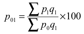
P 01 = (38720/31520)*100 = 122.84

 P 01 = ((34370/28020) + (38720/31520)) *100 = 122.66
2
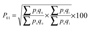
 P 01 = √ = ((34370/28020) + (38720/31520)) *100 = 122.69
Example 3
Commodity | Base year | Current year | ||
PO | QO | P1 | Q1 | |
A | 2 | 8 | 4 | 6 |
B | 5 | 10 | 6 | 5 |
C | 4 | 14 | 5 | 10 |
D | 2 | 19 | 2 | 13 |
Solution
Commodity | Base year | Current year |
|
|
|
| ||
PO | QO | P1 | Q1 | Poqo | P1qo | Poq1 | P1q1 | |
A | 2 | 8 | 4 | 6 | 16 | 32 | 12 | 24 |
B | 5 | 10 | 6 | 5 | 50 | 60 | 25 | 30 |
C | 4 | 14 | 5 | 10 | 56 | 70 | 40 | 50 |
D | 2 | 19 | 2 | 13 | 38 | 38 | 26 | 26 |
|
|
|
|
| 160 | 200 | 103 | 130 |

P 01 = (200/160)*100 = 125

P 01 = (130/103)*100 = 126.21

 P 01 = ((200/160) + (130/103)) *100 = 125.6
2

 P 01 = √ = ((200/160) + (130/103)) *100 = 125.61

= (200+130)/(160+103) *100 = 125.48
Example 4 –
Calculate the price indices from the following data by applying (1) Laspeyre’s method (2) Paasche’s method and (3) Fisher ideal number by taking 2010 as the base year.
Commodity | 2010 | 2011 | ||
PO | QO | P1 | Q1 | |
A | 20 | 10 | 25 | 13 |
B | 50 | 8 | 60 | 7 |
C | 35 | 7 | 40 | 6 |
D | 25 | 5 | 35 | 4 |
Solution
Commodity | 2010 | 2011 |
|
|
|
| ||
PO | QO | P1 | Q1 | Poqo | P1qo | Poq1 | P1q1 | |
A | 20 | 10 | 25 | 13 | 200 | 250 | 260 | 325 |
B | 50 | 8 | 60 | 7 | 400 | 480 | 350 | 420 |
C | 35 | 7 | 40 | 6 | 245 | 280 | 210 | 240 |
D | 25 | 5 | 35 | 4 | 125 | 175 | 100 | 140 |
|
|
|
|
| 970 | 1185 | 920 | 1125 |

P 01 = (1185/970)*100 = 122.16

P 01 = (1125/920)*100 = 122.28

 P 01 = √ = ((1185/970) + (1125/920)) *100 = 120.55
Example 5 –
Calculate the Dorbish and Bowley’s price index number for the following data taking 2014 as base year.
Item | 2010 | 2011 | ||
PO | QO | P1 | Q1 | |
Oil | 80 | 3 | 100 | 4 |
Pulses | 35 | 2 | 45 | 3 |
Sugar | 25 | 2 | 30 | 3 |
Rice | 50 | 30 | 54 | 35 |
Solution
Item | 2010 | 2011 |
|
|
|
| ||
PO | QO | P1 | Q1 | Poqo | P1qo | Poq1 | P1q1 | |
Oil | 80 | 3 | 100 | 4 | 240 | 300 | 320 | 400 |
Pulses | 35 | 2 | 45 | 3 | 70 | 90 | 105 | 135 |
Sugar | 25 | 2 | 30 | 3 | 50 | 60 | 75 | 90 |
Rice | 50 | 30 | 54 | 35 | 1500 | 1620 | 1750 | 1890 |
|
|
|
|
| 1860 | 2070 | 2250 | 2515 |

 P 01 = ((2070/1860) + (2515/2250)) *100 = 111.38
2
Example 6 –
Calculate a suitable price index from the following data
commodity | Quantity | price | |
|
| 2007 | 2010 |
X | 25 | 3 | 4 |
Y | 12 | 5 | 7 |
Z | 10 | 6 | 5 |
Solution
commodity | Q | P0 | P1 | P0Q | P1Q |
X | 25 | 3 | 4 | 75 | 100 |
Y | 12 | 5 | 7 | 60 | 84 |
Z | 10 | 6 | 5 | 60 | 50 |
|
|
|
| 195 | 234 |
Kelly price index

= 235/195*100 = 120
4. Weighted average of relative method – in this method different weights are used for the items according to their relative importance. If p = [p1/ p0] × 100 is the price relative index and w = p0q0 is attached to the commodity

Where,  means sum of weights for different commodities
 Sum of price relatives
Example 1 –
Commodity | Weight | Base price year | current price year |
A | 5 | 10 | 20 |
B | 4 | 15 | 25 |
C | 2 | 40 | 60 |
D | 3 | 25 | 40 |
Solution
Commodity | Weight | Base price year | current price year | price relatives | RW |
A | 5 | 10 | 20 | 20/10*100 = 200 | 1000 |
B | 4 | 15 | 25 | 25/15*100 =166.7 | 666.8 |
C | 2 | 40 | 60 | 60/40*100 = 150 | 300 |
D | 3 | 25 | 40 | 40/25*100 = 160 | 480 |
| 14 |
|
|
| 2446.8 |

P01 = 2446.8/14 = 174.8
Example 2 – compute price index by applying weighted average of relative method
Commodity | Quantity | Base price year | current price year |
Wheat | 20 | 3 | 4 |
Flour | 40 | 1.5 | 1.6 |
Milk | 10 | 1 | 1.5 |
Solution
Commodity | Quantity | Base price year | current price year | Weight | price relatives | RW |
Wheat | 20 | 3 | 4 | 60 | 133.3 | 8000 |
Flour | 40 | 1.5 | 1.6 | 60 | 106.7 | 6400 |
Milk | 10 | 1 | 1.5 | 10 | 150.0 | 1500 |
|
|
|
|
|
|
|
|
|
|
| 130 |
| 15900 |

P01 = 15900/130 = 122.30
Example 3 – Calculate weighted average of relative method
Commodity | Base price year | current price year | Weight |
x | 3 | 4 | 7 |
y | 1.5 | 1.6 | 8 |
z | 1 | 1.5 | 9 |
Solution
Commodity | Base price year | current price year | Weight | price relatives | RW |
x | 3 | 4 | 7 | 133.3 | 933.33 |
y | 1.5 | 1.6 | 8 | 106.7 | 853.33 |
z | 1 | 1.5 | 9 | 150.0 | 1350 |
|
|
| 24 |
| 3136.66 |

P01 = 3136.66/24 = 130.67
Reversibility test – time and factor
Index numbers are studied to know the relative changes in price and quantity for any two years compared. There are two tests which are used to test the adequacy for an index number. The two tests are as follows,
(i) Time Reversal Test
(ii) Factor Reversal Test
The criterion for a good index number is to satisfy the above two tests.
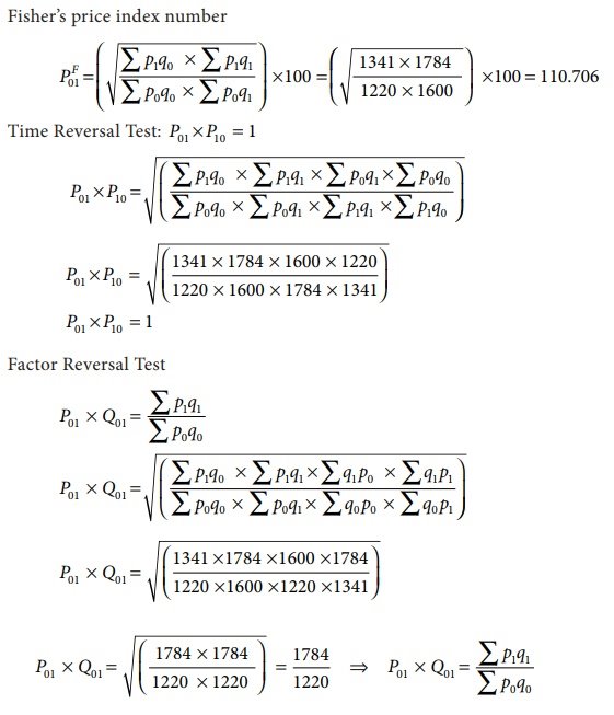
Time Reversal Test
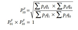
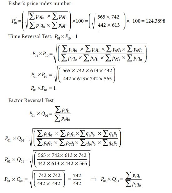
It is an important test for testing the consistency of a good index number. This test maintains time consistency by working both forward and backward with respect to time (here time refers to base year and current year). Symbolically the following relationship should be satisfied, P01 × P10 =1
Fisher’s index number formula satisfies the above relationship

when the base year and current year are interchanged, we get
Factor Reversal Test
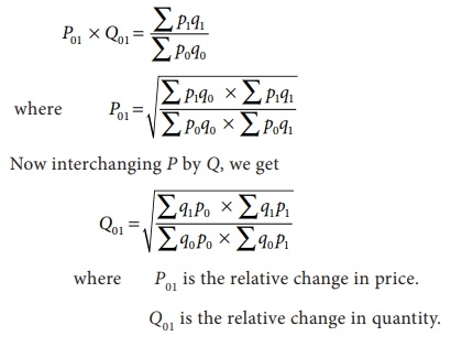
This is another test for testing the consistency of a good index number. The product of price index number and quantity index number from the base year to the current year should be equal to the true value ratio. That is, the ratio between the total value of current period and total value of the base period is known as true value ratio. Factor Reversal Test is given by,
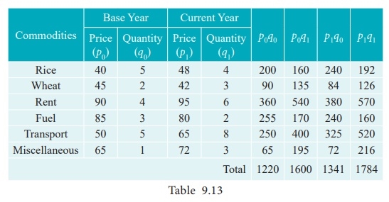
Example 1
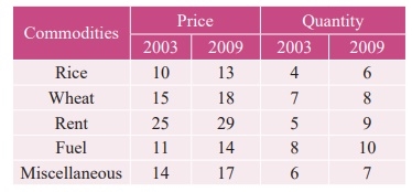
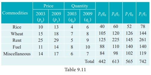
Calculate Fisher’s price index number and show that it satisfies both Time Reversal Test and Factor Reversal Test for data given below.
Solution
Example 2
Calculate Fisher’s price index number and show that it satisfies both Time Reversal Test and Factor Reversal Test for data given below.
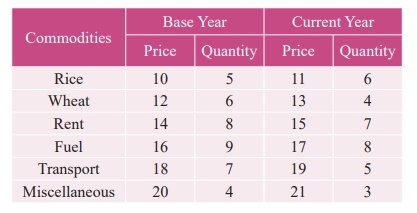
Solution
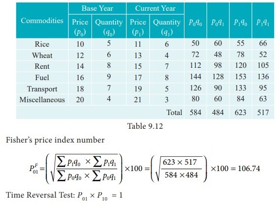
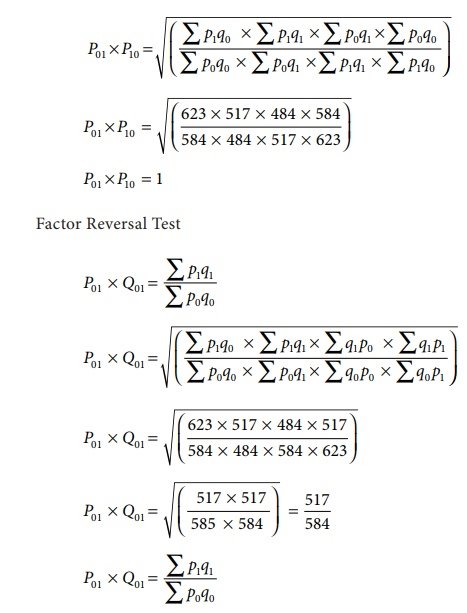
Example 3
Construct Fisher’s price index number and prove that it satisfies both Time Reversal Test and Factor Reversal Test for data following data.
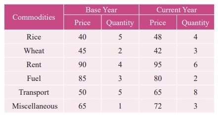
Solution
Key takeaways –
Reference


