Unit - 4

Data Mining Tasks

4.1 Introduction to Data Mining

• The data mining tasks can be classified generally into two types based on what a specific task tries to achieve. Those two categories are descriptive tasks and predictive tasks.

• The descriptive data mining tasks characterize the general properties of data whereas predictive data mining tasks perform inference on the available data set to predict how a new data set will behave.

Different Data Mining Tasks:-

• There are a number of data mining tasks such as classification, prediction, time-series analysis, association, clustering, summarization etc.

• All these tasks are either predictive data mining tasks or descriptive data mining tasks. A data mining system can execute one or more of the above specified tasks as part of data mining.

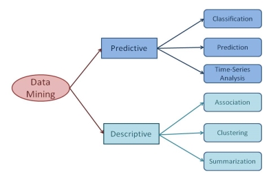
Fig 1: Data Mining Tasks

• Predictive data mining tasks come up with a model from the available data set that is helpful in predicting unknown or future values of another data set of interest.

• A medical practitioner trying to diagnose a disease based on the medical test results of a patient can be considered as a predictive data mining task

• . Descriptive data mining tasks usually finds data describing patterns and comes up with new, significant information from the available data set.

• A retailer trying to identify products that are purchased together can be considered as a descriptive data mining task.

A)    Classification:-

• Classification derives a model to determine the class of an object based on its attributes. A collection of records will be available, each record with a set of attributes.

• One of the attributes will be class attribute and the goal of classification task is assigning a class attribute to new set of records as accurately as possible.

• Classification can be used in direct marketing that is to reduce marketing costs by targeting a set of customers who are likely to buy a new product.

• Using the available data, it is possible to know which customers purchased similar products and who did not purchase in the past. Hence, {Purchase, don’t purchase} decision forms the class attribute in this case.

• Once the class attribute is assigned, demographic and lifestyle information of customers who purchased similar products can be collected and promotion mails can be sent to them directly.

B) Prediction:-

• Prediction task predicts the possible values of missing or future data. Prediction involves developing a model based on the available data and this model is used in predicting future values of a new data set of interest.

• For example, a model can predict the income of an employee based on education, experience and other demographic factors like place of stay, gender etc.

• Also prediction analysis is used in different areas including medical diagnosis, fraud detection etc.

C) Time - Series Analysis:-

• Time series is a sequence of events where the next event is determined by one or more of the preceding events.

• Time series reflects the process being measured and there are certain components that affect the behavior of a process.

• Time series analysis includes methods to analyze time-series data in order to extract useful patterns, trends, rules and statistics. Stock market prediction is an important application of time- series analysis.

D) Association:-

• Association discovers the association or connection among a set of items. Association identifies the relationships between objects.

• Association analysis is used for commodity management, advertising, catalog design, direct marketing etc.

• A retailer can identify the products that normally customers purchase together or even find the customers who respond to the promotion of same kind of products.

• If a retailer finds that beer and nappy are bought together mostly, he can put nappies on sale to promote the sale of beer.

E) Clustering:-

• Clustering is used to identify data objects that are similar to one another. The similarity can be decided based on a number of factors like purchase behavior, responsiveness to certain actions, geographical locations and so on.

• For example, an insurance company can cluster its customers based on age, residence, income etc. This group information will be helpful to understand the customers better and hence provide better customized services.

F) Summarization:-

• Summarization is the generalization of data. A set of relevant data is summarized which result in a smaller set that gives aggregated information of the data.

• For example, the shopping done by a customer can be summarized into total products, total spending, offers used, etc.

• Such high level summarized information can be useful for sales or customer relationship team for detailed customer and purchase behavior analysis.

• Data can be summarized in different abstraction levels and from different angles.

Key Takeaways

• Different data mining tasks are the core of data mining process. Different prediction and classification data mining tasks actually extract the required information from the available data sets.

4.2 Logistic Regression and Association Rules Analysis: -

• Logistic regression has been widely used in many academic areas and applications. It has been used to explore relationships among variables and to predict response classes based on explanatory variable values.

• It was initially used in biomedical studies (Agresti,2002); however, in recent decades it has been widely used in a number of other areas.

• In business, it has been used in applications involving credit scoring (Patra et al. 2008) and business forecasting and assessment (Lawson and Montgomery 2007; Lin et al. 2007).

• Other application areas include genetics (Coffey et al. 2004; Park and Hassie 2008), education (Morrell and Auer 2007), agriculture (Miramontes et al. 2006), engineering (Loh 2006; Kaur and Pulugurta 2008), neuroscience (Lu et al. 2004), and forestry (Yang et al. 2006; Yang et al. 2006).

• A logistic regression model explains the functional relationship between a link function and predictors in a linear form. The difference between the linear model and the logistic regression model is that whereas the linear model uses an identity link function, the logistic regression uses a logit link function.

• The logistic regression model uses a combination of categorical responses and explanatory variables, the latter of which can be quantitative variables, categorical variables, or both. The logistic regression model with only main effects is illustrated here:

Logit(p) = ln(p/1-p)= β0 + β1X1 + …. + βkXk

Where p is the probability of success, X’s are the main effects, and β’s are the coefficients of these main effects.

• Interactions have been addressed in different ways, especially interactions between categorical variables. According to Agresti (2002), interactions are typically omitted from classical logistic regression models.

• In other methods, interactions have been considered, but only after their main effects have been added to the model. Hosmer and Lemeshow (1989) considered interactions to be of interest after including main effects using the stepwise regression method.

• This type of analysis has two stages: the first stage considers only the main effects, and the second stage considers interactions among the significant main effects obtained in the first stage.

• Note that some applications allow models to add interactions without their main effects (Lin et al. 2008).

• In our study, we consider interactions and main effects simultaneously in the logistic regression model.

• As the number of interactions increases at an accelerated rate as the number of main effects increases, the subset selection method is extremely inefficient when all interactions are considered at the same time

• . Therefore, an efficient method for selecting potential interaction variables is required. We propose to implement association rules analysis for this purpose.

• Association rules analysis is a methodology for exploring relationships among items in the form of rules.

• Each rule has two parts. The first part includes left-hand side item(s), or condition(s), and the second part is a right-hand side item, or a result. The rule is always represented as a statement: if condition then result (Berry and Linoff 1997).

• Two measurements are attached to each rule. The first measurement is called support (s), and it is computed by

s = P (condition and result).

The second measurement is called confidence (c), and it is computed by

c = P (condition and result) /P (condition)

• . Association rules analysis finds all the rules that meet two key thresholds: minimum support and minimum confidence (Agrawal and Srikant 1994).

• This technique is widely used in market basket analysis. Here, the items for association rules analysis are products (e.g., milk, bread, and cheese). In this case, the rule would be “If a person buys bread (denoted in the condition by A), then the person will buy milk (denoted in the result by B).”

• The rule can be rewritten as “if A then B.” The support and confidence for this rule are s = P(A ⋂ B) and c = P(A ⋂B)/ P(A) = P(B/ A) , respectively.

• On the other hand, if the rule is “if B then A,” the support and confidence are s = P(A ⋂ B) and c = P(A ⋂ B)/ P(B) = P(A /B) , respectively. The information from this set of rules can then be used for product management (e.g., deciding which products to display together). It is well known that when the rule “if A then B” has confidence c, then the rule “if A then not B” will have confidence 1-c. Thus, when c is very small, the rule “if A then B” will not be considered. The rule “if A then not B” should be considered, however.

• This set of rules can be used for other purposes, including classification. A technique called classification rule mining (CRM), which is a subset of association rules analysis, was developed to find a set of rules in a database that would form an accurate classifier (Liu et al. 1998; Quinlan 1992). This technique uses an item to represent a pair consisting of a main effectand its corresponding integer value.

• More specific than association rules analysis, CRM has only one target, and this must be specified in advance. In general, the target of CRM is the response, which means the result of the rule (the right-hand side item) can only be the response and its class.

• Therefore, the left-hand side item (the condition) consists of the explanatory variable and its level.

• For example, assume there are k binary factors, X1, X2, …, Xk, and a binary response,Y. All variables have two levels denoted by 0 and 1. Many rules can be generated by CRM. One of the rules could be “if X1 = 1, then Y = 1” with s = P(X1 = 1 and Y = 1) and c = P(X1 = 1 and Y = 1) / P(X1 = 1).

• Another possibility is that the rule could be “if X1 = 1, then Y = 0” with s =

P(X1 = 1 and Y = 0) and c = P(X1 = 1 and Y = 0) / P(X1 = 1), among others.

• To our knowledge, few studies have linked association rules analysis to logistic regression modeling. Freyberger et al. (2004) apply classification rules mining to aid in the selection of logistic regression terms in transfer models of student learning.

• They begin a sequential search algorithm by choosing sets of main effects with high confidence for response prediction to create the first sets of logistic regression models.

• Then, rule variables that help predict the response from the misclassification instances are added.

• The process is repeated until adding new association rules no longer improves the misclassification rate. Cen et al. (2005) use a similar approach in their search for a cognitive model of student learning.

• In addition, Jaroszewicz (2006) applies association rules analysis in order to find polynomial terms to add to logistic regression.

• Unlike previous work, our proposed method applies association rules analysis as part of the global search for the logistic regression model (Changpetch and Lin 2012).

• In our study, we apply classification rule mining in order to retain only the potentially significant variables for consideration in building the logistic regression model.

• This methodology is an important aspect of the variables selection in our process. The proposed method creates a rule conversion technique for transforming important rules into binary variables and performing a global search for the optimal model.

• Several studies connect logistic regression and association rules analysis in support of achieving other objectives.

• For example, Shaharanee et al. (2009) apply logistic regression as a tool for finding significant rules in association rules analysis. Kamei et al. (2008) apply logistic regression with association rules analysis to create the fault-prone module prediction framework.

• The modules can be classified using a logistic regression model or association rules analysis, depending on the conditions of the modules themselves.

• Here, we are more interested in applying association rules analysis in order to find an optimal logistic model and to thereby facilitate understanding of datasets and improve model fit.

• There is a large body of research in the computer science literature that focuses on the different aspects, such as the accuracy of the classification method.

• However, our focus is on presenting our proposed method clearly; therefore, such issues will not be discussed further here.

Key Takeaways

• Logistic regression has been widely used in many academic areas and applications. It has been used to explore relationships among variables and to predict response classes based on explanatory variable values.

• The logistic regression model uses a combination of categorical responses and explanatory variables, the latter of which can be quantitative variables, categorical variables, or both. The logistic regression model with only main effects is illustrated here:

Logit(p) = ln(p/1-p)= β0 + β1X1 + …. + βkXk

• The first measurement is called support (s), and it is computed by

s = P (condition and result).

• The second measurement is called confidence (c), and it is computed by

c = P (condition and result) /P (condition)

4.3 Structure of Regression Model:

A regression problem is when the output variable is a real or continuous value, such as “salary” or “weight”. Many different models can be used, the simplest is the linear regression. It tries to fit data with the best hyperplane which goes through the points.

4.3.1 Regression Analysis: -

• It is a statistical process for estimating the relationships between the dependent variables or criterion variables and one or more independent variables or predictors.

• Regression analysis explains the changes in criterions in relation to changes in select predictors.

• The conditional expectation of the criterions based on predictors where the average value of the dependent variables is given when the independent variables are changed. Three major uses for regression analysis are determining the strength of predictors, forecasting an effect, and trend forecasting.

4.3.2 Types of Regression –

• Linear regression

• Logistic regression

• Polynomial regression

• Stepwise regression

• Stepwise regression

• Ridge regression

• Lasso regression

• ElasticNet regression

• Linear regression:-

Linear regression is used for predictive analysis. Linear regression is a linear approach for modeling the relationship between the criterion or the scalar response and the multiple predictors or explanatory variables. Linear regression focuses on the conditional probability distribution of the response given the values of the predictors. For linear regression, there is a danger of overfitting. The formula for linear regression is:

Y’ = bX + A.

• Logistic regression:-

Logistic regression is used when the dependent variable is dichotomous. Logistic regression estimates the parameters of a logistic model and is form of binomial regression. Logistic regression is used to deal with data that has two possible criterions and the relationship between the criterions and the predictors. The equation for logistic regression is:

l = β0 +  β1x1  + β2x2

• Polynomial regression :-

Polynomial regression is used for curvilinear data. Polynomial regression is fit with the method of least squares. The goal of regression analysis to model the expected value of a dependent variable y in regards to the independent variable x.

• Stepwise regression:-

Stepwise regression is used for fitting regression models with predictive models. It is carried out automatically. With each step, the variable is added or subtracted from the set of explanatory variables. The approaches for stepwise regression are forward selection, backward elimination, and bidirectional elimination.

• Ridge regression:-

Ridge regression is a technique for analyzing multiple regression data. When multicollinearity occurs, least squares estimates are unbiased. A degree of bias is added to the regression estimates, and a result, ridge regression reduces the standard errors.

• Lasso regression:-

Lasso regression is a regression analysis method that performs both variable selection and regularization. Lasso regression uses soft thresholding. Lasso regression selects only a subset of the provided covariates for use in the final model.

• ElasticNet regression:-

Elasticnet regression is a regularized regression method that linearly combines the penalties of the lasso and ridge methods. ElasticNet regression is used for support vector machines, metric learning, and portfolio optimization.

4.4 Single Linear Regression: -

• Simple linear regression is used to find out the best relationship between a single input variable (predictor, independent variable, input feature, and input parameter) & output variable (predicted, dependent variable, output feature, output parameter) provided that both variables are continuous in nature.

• This relationship represents how an input variable is related to the output variable and how it is represented by a straight line.

• To understand this concept, let us have a look at scatter plots. Scatter diagrams or plots provide a graphical representation of the relationship of two continuous variables.          

• After looking at scatter plot we can understand:

1. The direction

2. The strength

3. The linearity

• The above characteristics are between variable Y and variable X. The above scatter plot shows us that variable Y and variable X possess a strong positive linear relationship. Hence, we can project a straight line which can define the data in the most accurate way possible.

• If the relationship between variable X and variable Y is strong and linear, then we conclude that particular independent variable X is the effective input variable to predict dependent variable Y.

• To check the collinearity between variable X and variable Y, we have correlation coefficient (r), which will give you numerical value of correlation between two variables.

• You can have strong, moderate or weak correlation between two variables. Higher the value of “r”, higher the preference given for particular input variable X for predicting output variable Y. Few properties of “r” are listed as follows:

1. Range of r: -1 to +1

2. Perfect positive relationship: +1

3. Perfect negative relationship: -1

4. No Linear relationship: 0

5.Strong correlation: r > 0.85 (depends on business scenario)

Command used for calculation “r” in RStudio is:

> cor(X, Y)

Where, X: independent variable & Y: dependent variable Now, if the result of the above command is greater than 0.85 then choose simple linear regression.

• If r < 0.85 then use transformation of data to increase the value of “r” and then build a simple linear regression model on transformed data.

4.4.1 Steps to Implement Simple Linear Regression:-

• Analyze data (analyze scatter plot for linearity)

• Get sample data for model building

• Then design a model that explains the data

• And use the same developed model on the whole population to make predictions.

• The equation that represents how an independent variable X is related to a dependent variable Y.

• Y=bita0+bita1*x+£

Key Takeaways

• It is a statistical process for estimating the relationships between the dependent variables or criterion variables and one or more independent variables or predictors. Regression analysis explains the changes in criterions in relation to changes in select predictors.
• . For linear regression, there is a danger of overfitting. The formula for linear regression is:

Y’ = bX + A.

• . The equation for logistic regression is:

l = β0 + β1x1 + β2x2

4.5 Multiple Linear Regression:

• Regression models are used to describe relationships between variables by fitting a line to the observed data. Regression allows you to estimate how a dependent variable changes as the independent variable(s) change.

• Multiple linear regression is used to estimate the relationship between two or more independent variables and one dependent variable. You can use multiple linear regression when you want to know:

1. How strong the relationship is between two or more independent variables and one dependent variable (e.g. How rainfall, temperature, and amount of fertilizer added affect crop growth).

2. The value of the dependent variable at a certain value of the independent variables (e.g. The expected yield of a crop at certain levels of rainfall, temperature, and fertilizer addition

4.5.1 Assumptions of multiple linear regression:-

Multiple linear regression makes all of the same assumptions as simple linear regression:

• Homogeneity of variance (homoscedasticity): the size of the error in our prediction doesn’t change significantly across the values of the independent variable.

• Independence of observations: - the observations in the dataset were collected using statistically valid methods, and there are no hidden relationships among variables.

In multiple linear regression, it is possible that some of the independent variables are actually correlated with one another, so it is important to check these before developing the regression model. If two independent variables are too highly correlated (r2 > ~0.6), then only one of them should be used in the regression model.

• Linearity: the line of best fit through the data points is a straight line, rather than a curve or some sort of grouping factor.

4.5.2 How to perform a multiple linear regression:-

Multiple linear regression formula

The formula for a multiple linear regression is:

​yi​=β0​+β1​xi1​+β2​xi2​+...+βp​xip​+ϵ

• y = the predicted value of the dependent variable

• B0 = the y-intercept (value of y when all other parameters are set to 0)

• B1X1= the regression coefficient (B1) of the first independent variable (X1) (a.k.a. The effect that increasing the value of the independent variable has on the predicted y value)

• … = do the same for however many independent variables you are testing

• BpXp = the regression coefficient of the last independent variable

• ϵ = model error (a.k.a. How much variation there is in our estimate of y)

• To find the best-fit line for each independent variable, multiple linear regression calculates three things:

1. The regression coefficients that lead to the smallest overall model error.

2. The t-statistic of the overall model.

3. The associated p-value (how likely it is that the t-statistic would have occurred by chance if the null hypothesis of no relationship between the independent and dependent variables was true).

• It then calculates the t-statistic and p-value for each regression coefficient in the model.

Key Takeaways

• Multiple linear regression is used to estimate the relationship between two or more independent variables and one dependent variable.

• Multiple linear regression makes all of the same assumptions as simple linear regression:

1. Homogeneity of variance

2. Independence of observations

• The formula for a multiple linear regression is:

Yi​=β0​+β1​xi1​+β2​xi2​+...+βp​xip​+ϵ

4.6 Classification-classification problem and models: -

• It is a Data analysis task, i.e. the process of finding a model that describes and distinguishes data classes and concepts.

• Classification is the problem of identifying to which of a set of categories (subpopulations), a new observation belongs to, on the basis of a training set of data containing observations and whose categories membership is known.

• Example: Before starting any Project, we need to check it’s feasibility. In this case, a classifier is required to predict class labels such as ‘Safe’ and ‘Risky’ for adopting the Project and to further approve it. It is a two-step process such as :

1. Learning Step (Training Phase):-

(Construction of Classification Model)

Different Algorithms are used to build a classifier by making the model learn using the training set available. The model has to be trained for the prediction of accurate results.

2. Classification Step:-

Model used to predict class labels and testing the constructed model on test data and hence estimate the accuracy of the classification rules.

4.6.1 Classification Problems:-

1 - Email Spam

• The goal is to predict whether an email is a spam and should be delivered to the Junk folder.

• There is more than one method of identifying a mail as a spam. A simple method is discussed.

• The raw data comprises only the text part but ignores all images. Text is a simple sequence of words which is the input (X). The goal is to predict the binary response Y: spam or not.

• The first step is to process the raw data into a vector, which can be done in several ways. The method followed here is based on the relative frequencies of most common words and punctuation marks in e-mail messages. A set of 57 such words and punctuation marks are pre-selected by researchers. This is where domain knowledge plays an important role.

• Given these 57 most commonly occurring words and punctuation marks, then, in every e-mail message we would compute a relative frequency for each word, i.e., the percentage of times this word appears with respect to the total number of words in the email message.

• In the current example, 4601 email messages were considered in the training sample. These e-mail messages were identified as either a good e-mail or spam after reading the emails and assuming implicitly that human decision is perfect (an arguable point!).

• Relative frequency of the 57 most commonly used words and punctuation based on this set of emails was constructed. This is an example of supervised learning as in the training data the response Y is known. 

• In the future when a new email message is received, the algorithm will analyze the text sequence and compute the relative frequency for these 57 identified words. This is the new input vector to be classified into spam or not through the learning algorithm

2 - Handwritten Digit Recognition

• The goal is to identify images of single digits 0 - 9 correctly.

• The raw data comprises images that are scaled segments from five-digit ZIP codes. In the diagram below every green box is one image. The original images are very small, containing only 16 × 16 pixels. For convenience the images below are enlarged, hence the pixelation or 'boxiness' of the numbers.

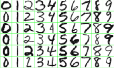
Fig 2: Handwritten Digit Recognition

• Every image is to be identified as 0 or 1 or 2 ... Or 9. Since the numbers are handwritten, the task is not trivial. For instance, a '5' sometimes can very much look like a '6', and '7' is sometimes confused with '1'.

• To the computer, an image is a matrix, and every pixel in the image corresponds to one entry in the matrix. Every entry is an integer ranging from a pixel intensity of 0 (black) to 255 (white).

• Hence the raw data can be submitted to the computer directly without any feature extraction. The image matrix was scanned row by row and then arranged into a large 256-dimensional vector.

• This is used as the input to train the classifier. Note that this is also a supervised learning algorithm where Y, the response, is multi-level and can take 10 values.

3 - Image segmentation

• Here is a more complex example of an image processing problem. The satellite images are to be identified into man-made or natural regions.

• For instance, in the aerial images shown below, buildings are labeled as man-made, and the vegetation areas are labeled as natural.

• These grayscale images are much larger than the previous example. These images are 512 × 512 pixels and again because these are grayscale images we can present pixel intensity with numbers 0 to 255.

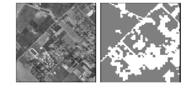
Fig 3: Image segmentation

• In the previous example of hand-written image identification, because of the small size of the images, no feature extraction was done. However in this problem feature extraction is necessary.

• A standard method of feature extraction in an image processing problem is to divide images into blocks of pixels or to form a neighborhood around each pixel.

• As is shown in the following diagram, after dividing the images into blocks of pixels or forming a neighborhood around each pixel, each block may be described by several features.

• As we have seen in the previous example, grayscale images can be represented by one matrix. Every entry in a greyscale image is an integer ranging from a pixel intensity of 0 (black) to 255 (white).

• Color images are represented by values of RGB (red, green and blue). Color images, therefore, are represented by 3 such matrices as seen below.

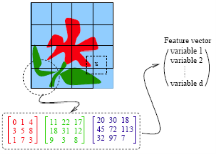
Fig 4: Color image Representation in RGB

• For each block, a few features (or statistics) may be computed using the color vectors for the pixels in the block. This set forms a feature vector for every block.

• Examples of features:

1. Average of R, G and B values for pixels in one block

2. Variance of the brightness of the pixels (brightness is the average of RGB color values). Small variance indicates the block is visually smooth.

3. The feature vectors for the blocks sometimes are treated as independent samples from an unknown distribution. Ignoring f the spatial dependence among feature vectors results in performance loss. To make the learning algorithm efficient the spatial dependence needs to be exploited. Only then the accuracy in classification will improve.

4 - Speech Recognition

• Another interesting example of data mining deals with speech recognition. For instance, if you call the University Park Airport, the system might ask you your flight number, or your origin and destination cities.

• The system does a very good job recognizing city names. This is a classification problem, in which each city name is a class. The number of classes is very big but finite.

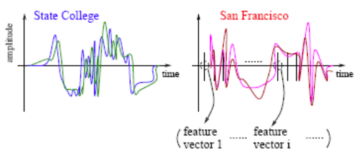
Fig 5: Speech Recognition

• The raw data involves voice amplitude sampled at discrete time points (a time sequence), which may be represented in the waveforms as shown above. In speech recognition, a very popular method is the Hidden Markov Model.

• At every time point, one or more features, such as frequencies, are computed. The speech signal essentially becomes a sequence of frequency vectors. This sequence is assumed to be an instance of a hidden Markov model (HMM). An HMM can be estimated using multiple sample sequences under the same class (e.g., city name).

5 - DNA Expression Microarray

• Our goal here is to identify disease or tissue types based on the gene expression levels.

• For each sample taken from a tissue of a particular disease type, the expression levels of a very large collection of genes are measured. The input data goes through a data cleaning process.

• Data cleaning may include but is certainly not limited to, normalization, elimination of noise and perhaps log-scale transformations. A large volume of literature exists on the topic of cleaning microarray data.

• In the example considered 96 samples were taken from 9 classes or types of tissues. It was expensive to collect the tissue samples, at least in the early days. Therefore, the sample size is often small but the dimensionality of data is very high.

• Every sample is measured on 4026 genes. Very often microarray data analysis has its own challenges with a small number of observations and very large number of features from each observation.

6 - DNA Sequence Classification

• Each genome is made up of DNA sequences and each DNA segment has specific biological functions. However there are DNA segments which are non-coding, i.e. they do not have any biological function (or their functionalities are not yet known).

• One problem in DNA sequencing is to label the sampled segments as coding or non-coding (with a biological function or without).

• The raw DNA data comprises sequences of letters, e.g., A, C, G, T for each of the DNA sequences.

• One method of classification assumes the sequences to be realizations of random processes. Different random processes are assum for different classes of sequences.

• In the above examples on classification, several simple and complex real-life problems are considered. Classification problems are faced in a wide range of research areas. The raw data can come in all sizes, shapes, and varieties.

• A critical step in data mining is to formulate a mathematical problem from a real problem. In this course, the focus is on learning algorithms. The formulation step is largely left out.

Key Takeaways

• Classification is the problem of identifying to which of a set of categories (subpopulations), a new observation belongs to, on the basis of a training set of data containing observations and whose categories membership is known.

• It is a two-step process such as :

1. Learning Step (Training Phase):-

2. Classification Step:-

4.7 Classification Tree: -

4.7.1 Introduction

• Classification tree methods (i.e., decision tree methods) are recommended when the data mining task contains classifications or predictions of outcomes, and the goal is to generate rules that can be easily explained and translated into SQL or a natural query language.

• A Classification tree labels, records, and assigns variables to discrete classes. A Classification tree can also provide a measure of confidence that the classification is correct.

• A Classification tree is built through a process known as binary recursive partitioning. This is an iterative process of splitting the data into partitions, and then splitting it up further on each of the branches.

• Initially, a Training Set is created where the classification label (i.e., purchaser or non-purchaser) is known (pre-classified) for each record. Next, the algorithm systematically assigns each record to one of two subsets on the some basis (i.e., income > $75,000 or income <= $75,000).

• The object is to attain an homogeneous set of labels (i.e., purchaser or non-purchaser) in each partition. This partitioning (splitting) is then applied to each of the new partitions.

• The process continues until no more useful splits can be found. The heart of the algorithm is the rule that determines the initial split rule (displayed in the following figure).

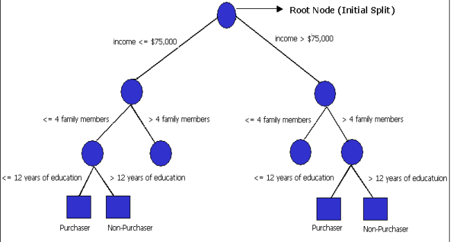
Fig 6: Hypothetical Classification Tree

• The process starts with a Training Set consisting of pre-classified records (target field or dependent variable with a known class or label such as purchaser or non-purchaser).

• The goal is to build a tree that distinguishes among the classes. For simplicity, assume that there are only two target classes, and that each split is a binary partition.

• The partition (splitting) criterion generalizes to multiple classes, and any multi-way partitioning can be achieved through repeated binary splits. To choose the best splitter at a node, the algorithm considers each input field in turn.

• In essence, each field is sorted. Every possible split is tried and considered, and the best split is the one that produces the largest decrease in diversity of the classification label within each partition (i.e., the increase in homogeneity). This is repeated for all fields, and the winner is chosen as the best splitter for that node. The process is continued at subsequent nodes until a full tree is generated.

• XLMiner uses the Gini index as the splitting criterion, which is a commonly used measure of inequality. The index fluctuates between a value of 0 and 1.

• A Gini index of 0 indicates that all records in the node belong to the same category. A Gini index of 1 indicates that each record in the node belongs to a different category.

• For a complete discussion of this index, please see Leo Breiman’s and Richard Friedman’s book, Classification and Regression Trees .

4.7.2 Pruning the Tree:-

• Pruning is the process of removing leaves and branches to improve the performance of the decision tree when moving from the Training Set (where the classification is known) to real-world applications (where the classification is unknown).

• The tree-building algorithm makes the best split at the root node where there are the largest number of records, and considerable information. Each subsequent split has a smaller and less representative population with which to work.

• Towards the end, idiosyncrasies of training records at a particular node display patterns that are peculiar only to those records. These patterns can become meaningless for prediction if you try to extend rules based on them to larger populations.

• For example, if the classification tree is trying to predict height and it comes to a node containing one tall person X and several other shorter people, the algorithm decreases diversity at that node by a new rule imposing people named X are tall, and thus classify the Training Data.

• In the real world, this rule is obviously inappropriate. Pruning methods solve this problem -- they let the tree grow to maximum size, then remove smaller branches that fail to generalize. (Note: Do not include irrelevant fields such as name, as this is simply used an illustration.)

• Since the tree is grown from the Training Set, when it has reaches full structure it usually suffers from over-fitting (i.e., it is explaining random elements of the Training Data that are not likely to be features of the larger population of data).

• This results in poor performance on data. Therefore, trees must be pruned using the Validation Set.

4.7.3 Ensemble Methods

1. XLMiner V2015 offers three powerful ensemble methods for use with Classification trees: bagging (bootstrap aggregating), boosting, and random trees.

2.     The Classification Tree Algorithm on its own can be used to find one model that results in good classifications of the new data.

3.     We can view the statistics and confusion matrices of the current classifier to see if our model is a good fit to the data, but how would we know if there is a better classifier waiting to be found? The answer is that we do not know if a better classifier exists.

4.     However, ensemble methods allow us to combine multiple weak classification tree models that, when taken together form a new, more accurate strong classification tree model.

5.     These methods work by creating multiple diverse classification models, taking different samples of the original data set, and then combining their outputs.

6.     Outputs may be combined by several techniques for example, majority vote for classification and averaging for regression.

7.     This combination of models effectively reduces the variance in the strong model.

8.     The three different type of ensemble methods offered in XLMiner (bagging, boosting, and random trees) differ on three items:

1) The selection of a Training Set for each classifier or weak model;

2) How the weak models are generated; and

3) How the outputs are combined.

In all three methods, each weak model is trained on the entire Training Set to become proficient in some portion of the data set.

9.     Bagging (bootstrap aggregating) was one of the first ensemble algorithms to be documented. It is a simple, effective algorithm.

10. Bagging generates several Training Sets by using random sampling with replacement (bootstrap sampling), applies the classification tree algorithm to each data set, then takes the majority vote between the models to determine the classification of the new data.

11. The biggest advantage of bagging is the relative ease with which the algorithm can be parallelized, which makes it a better selection for very large data sets.

12. Boosting builds a strong model by successively training models to concentrate on the misclassified records in previous models.

13. Once completed, all classifiers are combined by a weighted majority vote. XLMiner offers three different variations of boosting as implemented by the AdaBoost algorithm (ensemble algorithm): M1 (Freund), M1 (Breiman), and SAMME (Stagewise Additive Modeling using a Multi-class Exponential).

14. Adaboost.M1 first assigns a weight (wb(i)) to each record or observation. This weight is originally set to 1/n, and is updated on each iteration of the algorithm. An original classification tree is created using this first Training Set (Tb) and an error is calculated as

Where, the I() function returns 1 if true, and 0 if not.

15. The error of the classification tree in the bth iteration is used to calculate the constant ?b. This constant is used to update the weight (wb(i). In AdaBoost.M1 (Freund), the constant is calculated as

αb= ln((1-eb)/eb)

16. In AdaBoost.M1 (Breiman), the constant is calculated as

αb= 1/2ln((1-eb)/eb)

17. In SAMME, the constant is calculated as

αb= 1/2ln((1-eb)/eb + ln(k-1) where k is the number of classes

Where, the number of categories is equal to 2, SAMME behaves the same as AdaBoost Breiman.

18. In any of the three implementations (Freund, Breiman, or SAMME), the new weight for the (b + 1)th iteration will be

19. Afterwards, the weights are all readjusted to sum to 1. As a result, the weights assigned to the observations that were classified incorrectly are increased and the weights assigned to the observations that were classified correctly are decreased.

20. This adjustment forces the next classification model to put more emphasis on the records that were misclassified. (The constant is also used in the final calculation, which will give the classification model with the lowest error more influence.)

21.  This process repeats until b = Number of weak learners (controlled by the User). The algorithm then computes the weighted sum of votes for each class and assigns the winning classification to the record.

22. Boosting generally yields better models than bagging; however, it does have a disadvantage as it is not parallelizable. As a result, if the number of weak learners is large, boosting would not be suitable.

23. Random trees (i.e., random forests) is a variation of bagging. This method works by training multiple weak classification trees using a fixed number of randomly selected features (sqrt[number of features] for classification, and a number of features/3 for prediction), then takes the mode of each class to create a strong classifier.

24.  Typically, in this method the number of “weak” trees generated could range from several hundred to several thousand depending on the size and difficulty of the training set.

25. Random Trees are parallelizable since they are a variant of bagging. However, since Random Trees selects a limited amount of features in each iteration, the performance of random trees is faster than bagging.

26. Classification Tree Ensemble methods are very powerful methods, and typically result in better performance than a single tree.

27. This feature addition in XLMiner V2015 provides more accurate classification models and should be considered over the single tree method.

Key Takeaways

• Classification tree methods (i.e., decision tree methods) are recommended when the data mining task contains classifications or predictions of outcomes, and the goal is to generate rules that can be easily explained and translated into SQL or a natural query language.

• A Classification tree labels, records, and assigns variables to discrete classes. A Classification tree can also provide a measure of confidence that the classification is correct.

• A Classification tree is built through a process known as binary recursive partitioning.

• The goal is to build a tree that distinguishes among the classes.

• Pruning is the process of removing leaves and branches to improve the performance of the decision tree when moving from the Training Set (where the classification is known) to real-world applications (where the classification is unknown).

• XLMiner V2015 offers three powerful ensemble methods for use with Classification trees: bagging (bootstrap aggregating), boosting, and random trees

28. The Classification Tree Algorithm on its own can be used to find one model that results in good classifications of the new data.

4.8 Bayesian Classification:-

Bayesian classification is based on Bayes' Theorem. Bayesian classifiers are the statistical classifiers. Bayesian classifiers can predict class membership probabilities such as the probability that a given tuple belongs to a particular class.

4.8.1 Baye’s Theorem:-

Bayes' Theorem is named after Thomas Bayes. There are two types of probabilities −

1. Posterior Probability [P(H/X)]

2. Prior Probability [P(H)]

Where X is data tuple and H is some hypothesis.

29. According to Bayes' Theorem,

P(H/X)= P(X/H)P(H) / P(X)

4.8.2 Bayesian Belief Network:-

30. Bayesian Belief Networks specify joint conditional probability distributions. They are also known as Belief Networks, Bayesian Networks, or Probabilistic Networks.

31. A Belief Network allows class conditional independencies to be defined between subsets of variables.

32. It provides a graphical model of causal relationship on which learning can be performed.

33. We can use a trained Bayesian Network for classification.

34. There are two components that define a Bayesian Belief Network −

1. Directed acyclic graph

2. A set of conditional probability tables

4.8.3 Directed Acyclic Graph:-

35. Each node in a directed acyclic graph represents a random variable.

36. These variable may be discrete or continuous valued.

37. These variables may correspond to the actual attribute given in the data.

4.8.4 Directed Acyclic Graph Representation:-

• The following diagram shows a directed acyclic graph for six Boolean variables.

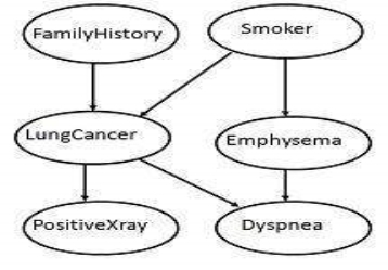
Fig 7: Acyclic Graph Example

• The arc in the diagram allows representation of causal knowledge. For example, lung cancer is influenced by a person's family history of lung cancer, as well as whether or not the person is a smoker.

• It is worth noting that the variable PositiveXray is independent of whether the patient has a family history of lung cancer or that the patient is a smoker, given that we know the patient has lung cancer.

4.8.5 Conditional Probability Table

• The conditional probability table for the values of the variable LungCancer (LC) showing each possible combination of the values of its parent nodes, FamilyHistory (FH), and Smoker (S) is as follows

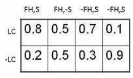
Fig 8: Conditional Probability Example

Key Takeaways

• Bayesian classification is based on Bayes' Theorem. Bayesian classifiers are the statistical classifiers. Bayesian classifiers can predict class membership probabilities such as the probability that a given tuple belongs to a particular class.

38. According to Bayes' Theorem,

P(H/X)= P(X/H)P(H) / P(X)

39. There are two components that define a Bayesian Belief Network −

1. Directed acyclic graph

2. A set of conditional probability tables

References:

1. Data mining Introductory and Advanced topics- Margaret H. Dunhum-Pearson

2.     Data Mining: Concepts and Techniques Second Edition- Jaiwei Han and Micheline kamber-Morgan KaufMan publisher

3.     Data Mining and Analysis Fundamental Concepts and Algorithms –Mohammed J. Zaki and Wager Meira Jr. Cambridge University Press.

4.     Business Intelligence – Data Mining and optimization for Decision Making – Curlo Vercellis-Wiley Publications.