UNIT 3
IMAGE RESTORATION
Image restoration is the operation of taking a corrupt/noisy image and estimating the clean, original image. Corruption may come in many forms such as motion blur, noise, and camera misfocus. Image restoration is performed by reversing the process that blurred the image and such is performed by imaging a point source and use the point source image, which is called the Point Spread Function (PSF) to restore the image information lost to the blurring process.
Image restoration is different from image enhancement in that the latter is designed to emphasize features of the image that make the image more pleasing to the observer, but not necessarily to produce realistic data from a scientific point of view. Image enhancement techniques (like contrast stretching or de-blurring by the nearest neighbor procedure) provided by imaging packages use no a priori model of the process that created the image.
With image, enhancement noise can effectively be removed by sacrificing some resolution, but this is not acceptable in many applications. In a fluorescence microscope, the resolution in the z-direction as bad as it is. More advanced image processing techniques must be applied to recover the object.
The objective of image restoration techniques is to reduce noise and recover resolution loss Image processing techniques are performed either in the image domain or the frequency domain. The most straightforward and conventional technique for image restoration is deconvolution, which is performed in the frequency domain and after computing the Fourier transform of both the image and the PSF and undo the resolution loss caused by the blurring factors. This deconvolution technique, because of its direct inversion of the PSF which typically has poor matrix condition number, amplifies noise and creates an imperfect deblurred image. Also, conventionally the blurring process is assumed to be shift-invariant. Hence more sophisticated techniques, such as regularized deblurring, have been developed to offer robust recovery under different types of noises and blurring functions. It is of 3 types: 1. Geometric correction 2. Radiometric correction 3. Noise removal
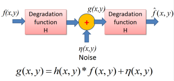
A model for the Image Degradation/Restoration process

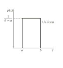
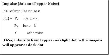
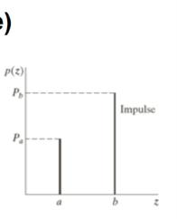
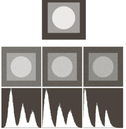
Noise Models
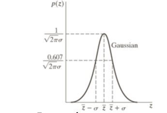
Gaussian Noise
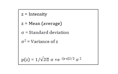
Mathematically tractable in both spatial and frequency domain. PDF of a Gaussian random variable z is given by
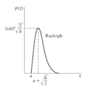
Rayleigh Noise
Displacement from origin
Skewed to the right


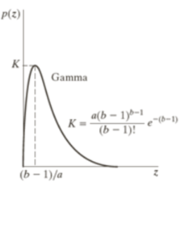
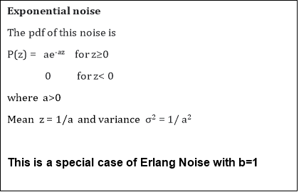
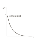
Erlang(gamma) noise







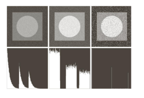
Periodic Noise
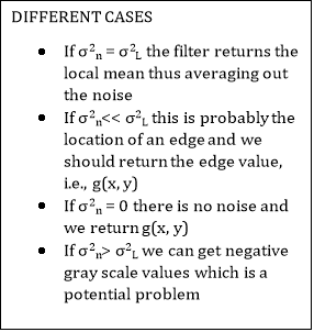
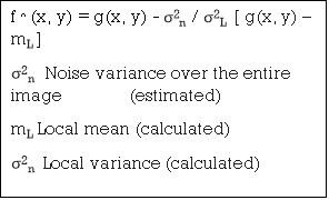
 Restoration in the presence of noise only-Spatial filtering
Key takeaway
Image restoration is the operation of taking a corrupt/noisy image and estimating the clean, original image. Corruption may come in many forms such as motion blur, noise, and camera misfocus. Image restoration is performed by reversing the process that blurred the image and such is performed by imaging a point source and use the point source image, which is called the Point Spread Function (PSF) to restore the image information lost to the blurring process.
Mean Filters
In this section, we discuss briefly the noise-reduction spatial filters introduced in Section 3.6 and develop several other filters whose performance is in many cases superior to the filters discussed in that section.
Arithmetic mean filter
 This is the simplest of the mean filters. Let Sxv represent the set of coordinates in a rectangular sub-image window of size m X n, centered at the point (x, y). The arithmetic means filtering process computes the average value of the corrupted image g(x, y) in the area defined by Sxy. The value of the restored image at any point (x, y) is simply the arithmetic mean computed using the pixels in the region defined by S. In other words.
This operation can be implemented using a convolution mask in which ail coefficients have a value of 1/mn. As discussed in Section 3.6.1, a mean filter simply smoothes local variations in an image. Noise is reduced as a result of blurring.
Geometric mean filter
 An image restored using a geometric mean filter is given by the expression
Here, each restored pixel is given by the product of the pixels in the sub-image window, raised to the power 1/mn. As shown in Example 52, a geometric mean filter achieves smoothing comparable to the arithmetic mean filter, but it tends to lose less image detail in the process.
Harmonic mean filter
 The harmonic mean filtering operation is given by the expression
The harmonic mean filter works well for salt noise but fails for pepper noise. It does well also with other types of noise like Gaussian noise.
Contraharmonic mean filter
 The contraharmonic mean filtering operation yields a restored image based on the expression
Where Q is called the order of the filter. This filter is well suited for reducing or virtually eliminating the effects of salt-and-pepper noise. For positive values of Q, the filter eliminates pepper noise. For negative values of Q, it eliminates salt noise. It cannot do both simultaneously. Note that the contra harmonic filter reduces to the arithmetic mean filter if Q = 0, and to the harmonic mean filter if Q = - 1
Order-Statistics Filters
Order-statistics filters were introduced in Section 3.6.2. We now expand the dis¬cussion in that section and introduce some additional order-statistics filters. As noted in Section 3.6.2, order-statistics filters are spatial filters whose response is based on ordering (ranking) the pixels contained in the image area encom¬passed by the filter. The response of the filter at any point is determined by the ranking result
Median filter
 The best-known order-statistics filter is the median filter, which, as its name implies, replaces the value of a pixel by the median of the gray levels in the neighborhood of that pixel:
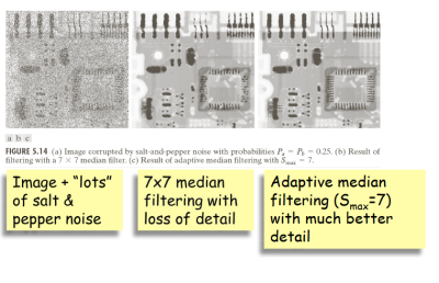
The original value of the pixel is included in the computation of the median. Median filters are quite popular because, for certain types of random noise, they provide excellent noise-reduction capabilities, with considerably less blurring than linear smoothing filters of similar size. Median filters are particularly effective in the presence of both bipolar and unipolar impulse noise. In fact, as Ex¬ample 5.3 shows, the median filter yields excellent results for images corrupted by this type of noise. Computation of the median and implementation of this filter are discussed in detail in Section 3.6.2.
Max and min filters
 Although the median filter is by far the order-statistics filter most used in image processing.it is by no means the only one. The median represents the 50th percentile of a ranked set of numbers, but the reader will recall from basic statis¬tics that ranking lends itself to many other possibilities. For example, using the 100th percentile results in the so-called max filter given by:
 This filter is useful for finding the brightest points in an image. Also, because pep¬per noise has very low values, it is reduced by this filter as a result of the max selection process in the sub-image area S. The 0th percentile filter is the Min filter.
Key takeaway
This is the simplest of the mean filters. Let Sxv represent the set of coordinates in a rectangular sub-image window of size m X n, centered at the point (x, y). The arithmetic means filtering process computes the average value of the corrupted image g(x, y) in the area defined by Sxy. The value of the restored image at any point (x, y) is simply the arithmetic mean computed using the pixels in the region defined by S.

The BANDREJECT_FILTER function applies a low-reject, high-reject, or band-reject filter on a one-channel image.
A band-reject filter is useful when the general location of the noise in the frequency domain is known. A band-reject filter blocks frequencies within the chosen range and lets frequencies outside of the range pass through.
The following diagrams give a visual interpretation of the transfer functions:
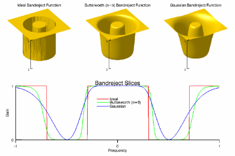
Fig 1 – Band reject
This routine is written in the IDL language. Its source code can be found in the file bandreject_filter.pro in the lib subdirectory of the IDL distribution.
Syntax
Result = BANDREJECT_FILTER( ImageData, LowFreq, HighFreq [, /IDEAL] [, BUTTERWORTH=value] [, /GAUSSIAN] )
Return Value
Returns a filtered image array of the same dimensions and type as ImageData.
Arguments
ImageData
A two-dimensional array containing the pixel values of the input image.
LowFreq
The lower limit of the cutoff frequency band. This value should be between 0 and 1 (inclusive) and must be less than HighFreq.
HighFreq
The upper limit of the cutoff frequency band. This value should be between 0 and 1 (inclusive) and must be greater than LowFreq.
Keywords
IDEAL
Set this keyword to use an ideal band-reject filter. In this type of filter, frequencies outside of the given range are passed without attenuation, and frequencies inside of the given range are blocked. This behavior makes the ideal band-reject filters very sharp.

 The centered Fast Fourier Transform (FFT) is filtered by the following function, where DL is the lower bound of the frequency band, DH is the upper bound of the frequency band, and D(u,v) is the distance between a point (u,v) in the frequency domain and the center of the frequency rectangle:
BUTTERWORTH
Set this keyword to the dimension of the Butterworth filter to apply to the frequency domain. With a Butterworth band-reject filter, frequencies at the center of the frequency band are completely blocked and frequencies at the edge of the band are attenuated by a fraction of the maximum value. The Butterworth filter does not have any sharp discontinuities between passed and filtered frequencies.
Note: The default for BANDREJECT_FILTER is BUTTERWORTH=1.
The centered FFT is filtered by one of the following functions, where D0 is the center of the frequen

Cy band, W is the width of the frequency band, D=D(u,v) is the distance between a point (u,v) in the frequency domain and the center of the frequency rectangle, and n is the dimension of the Butterworth filter:
Note: A low Butterworth dimension is close to Gaussian, and a high Butterworth dimension is close to Ideal.
GAUSSIAN
Set this keyword to use a Gaussian band-reject filter. In this type of filter, the transition between unfiltered and filtered frequencies is very smooth.
 The centered FFT is filtered by one of the following functions, where D0 is the center of the frequency band, W is the width of the frequency band, and D=D(u,v) is the distance between a point (u,v) in the frequency domain and the center of the frequency rectangle:
Examples
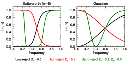
Here, we plot the frequency response of the Butterworth (n=5) and Gaussian filters. For the low-reject filter we use a high-frequency cutoff of 0.5, for high-reject we use a cutoff of 0.5, and for the band-reject we use DL=0.2 and DH=0.6.
m = [0.2,0.27,0.05,0.1]
p = PLOT('1-1/(1 + (X/0.5)^10)', '3', DIM=[600,300], FONT_SIZE=10, $
XRANGE=[0,1], YRANGE=[0,1.1], LAYOUT=[2,1,1], MARGIN=m, $
XTITLE='frequency', YTITLE='H(u,v)', TITLE='Butterworth (n=5)')
p = PLOT('1/(1 + (X*0.4/(X^2-0.4^2))^10)', '3g', /OVERPLOT)
p = PLOT('1-1/(1 + (0.5/X)^10)', '3r', /OVERPLOT)
p = PLOT('1-exp(-X^2/(2*0.5^2))', '3', DIM=[600,300], FONT_SIZE=10, $
XRANGE=[0,1], YRANGE=[0,1.1], LAYOUT=[2,1,2], MARGIN=m, $
XTITLE='frequency', YTITLE='H(u,v)', TITLE='Gaussian', /CURRENT)
p = PLOT('1-exp(-((X^2-0.4^2)/(X*0.4))^2)', '3g', /OVERPLOT)
p = PLOT('exp(-X^2/(2*0.5^2))', '3r', /OVERPLOT)
t = TEXT(0.12,0.05,'Low-reject $D_H=0.5$',/NORM, FONT_SIZE=9)
t = TEXT(0.38,0.05,'High-reject $D_L=0.5$',COLOR='red',/NORM, FONT_SIZE=9)
t = TEXT(0.64,0.05,'Band-reject $D_L=0.2, D_H=0.6$', $
COLOR='green',/NORM, FONT_SIZE=9)
p.Save, 'bandreject_filter.png', resolution=120
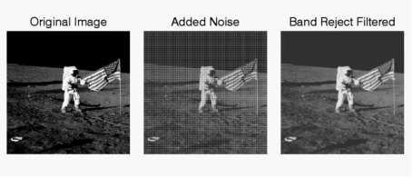
In the following example, we add some sinusoidal noise to an image and filter it with BANDREJECT_FILTER.
; Read in the file
File = FILEPATH('moon_landing.png', SUBDIR=['examples','data'])
ImageOriginal = READ PNG(file)
; Generate some sinusoidal noise
XCoords = LINDGEN(300,300) MOD 300
YCoords = TRANSPOSE(xCoords)
Noise = -SIN(xCoords*1.5)-SIN(yCoords*1.5)
ImageNoise = imageOriginal + 50*noise
; Filter the noise with a band reject filter
ImageFiltered = BRANDREJECT FILTER(imageNoise, 0.28, 0.38)
; Display the original, noise-added, and filtered images
i=IMAGE(imageOriginal, LAYOUT=[3,1,1], TITLE='Original Image', $
DIMENSIONS=[700,300])
i=IMAGE(imageNoise, LAYOUT=[3,1,2], /CURRENT, TITLE='Added Noise')
i=IMAGE(imageFiltered, LAYOUT=[3,1,3], /CURRENT, $
TITLE='Band Reject Filtered')
i.Save, 'bandreject_filter_ex.gif', resolution=120
Key takeaway
The BANDREJECT_FILTER function applies a low-reject, high-reject, or band-reject filter on a one-channel image.
A band-reject filter is useful when the general location of the noise in the frequency domain is known. A band-reject filter blocks frequencies within the chosen range and lets frequencies outside of the range pass through.
The BANDPASS_FILTER function applies a lowpass, bandpass, or highpass filter to a one-channel image.
A bandpass filter is useful when the general location of the noise in the frequency domain is known. The bandpass filter allows frequencies within the chosen range through and attenuates frequencies outside of the given range.
The following diagrams give a visual interpretation of the transfer functions:
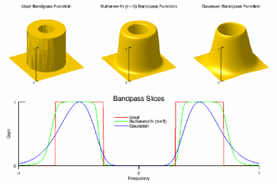
Fig 2 – Bandpass
This routine is written in the IDL language. Its source code can be found in the file bandpass_filter.pro in the lib subdirectory of the IDL distribution.
Syntax
Result = BANDPASS_FILTER( ImageData, LowFreq, HighFreq [, /IDEAL] [, BUTTERWORTH=value] [, /GAUSSIAN] )
Return Value
Returns a filtered image array of the same dimensions and type as ImageData.
Arguments
ImageData
A two-dimensional array containing the pixel values of the input image.
LowFreq
The lower limit of the pass-through frequency band. This value should be between 0 and 1 (inclusive) and must be less than HighFreq.
HighFreq
The upper limit of the pass-through frequency band. This value should be between 0 and 1 (inclusive) and must be greater than LowFreq.
Keywords
IDEAL
Set this keyword to use an ideal bandpass filter. Ideal bandpass filters, frequencies within the given range are passed through without attenuation, and frequencies outside of the given range are completely removed. This behavior makes ideal bandpass filters very sharp.

 The centered Fast Fourier Transform (FFT) is filtered by the following function, where DL is the lower bound of the frequency band, DH is the upper bound of the frequency band, and D(u,v) is the distance between a point (u,v) in the frequency domain and the center of the frequency rectangle:
BUTTERWORTH
Set this keyword to the dimension of the Butterworth filter to apply to the frequency domain. With a Butterworth bandpass filter, frequencies at the center of the frequency band are unattenuated and frequencies at the edge of the band are attenuated by a fraction of the maximum value. The Butterworth filter does not have sharp discontinuities between frequencies that are passed and filtered.
The default for BANDPASS_FILTER is BUTTERWORTH=1.
 The centered FFT is filtered by one of the following functions, where D0 is the center of the frequency band, W is the width of the frequency band, D=D(u,v) is the distance between a point (u,v) in the frequency domain and the center of the frequency rectangle, and n is the dimension of the Butterworth filter:
A low Butterworth dimension is close to Gaussian, and a high Butterworth dimension is close to Ideal.
GAUSSIAN
Set this keyword to use a Gaussian bandpass filter. In this type of filter, the transition between unfiltered and filtered frequencies is very smooth.
 The centered FFT is filtered by one of the following functions, where D0 is the center of the frequency band, W is the width of the frequency band, and D=D(u,v) is the distance between a point (u,v) in the frequency domain and the center of the frequency rectangle:
Examples
Here, we plot the frequency response of the Butterworth (n=5) and Gaussian filters. For the lowpass filter we use a high-frequency cutoff of 0.5, for highpass we use a cutoff of 0.5, and for the bandpass we use DL=0.2 and DH=0.8.
m = [0.2,0.27,0.05,0.1]
p = PLOT('1/(1 + (X/0.5)^10)', '3', DIM=[600,300], FONT_SIZE=10, $
XRANGE=[0,1], YRANGE=[0,1.1], LAYOUT=[2,1,1], MARGIN=m, $
XTITLE='frequency', YTITLE='H(u,v)', TITLE='Butterworth (n=5)')
p = PLOT('1-1/(1 + (X*0.6/(X^2-0.5^2))^10)', '3g', /OVERPLOT)
p = PLOT('1/(1 + (0.5/X)^10)', '3r', /OVERPLOT)
p = PLOT('exp(-X^2/(2*0.5^2))', '3', DIM=[600,300], FONT_SIZE=10, $
XRANGE=[0,1], YRANGE=[0,1.1], LAYOUT=[2,1,2], MARGIN=m, $
XTITLE='frequency', YTITLE='H(u,v)', TITLE='Gaussian', /CURRENT)
p = PLOT('exp(-((X^2-0.5^2)/(X*0.6))^2)', '3g', /OVERPLOT)
p = PLOT('1-exp(-X^2/(2*0.5^2))', '3r', /OVERPLOT)
t = TEXT(0.15,0.05,'Lowpass $D_H=0.5$',/NORM, FONT_SIZE=9)
t = TEXT(0.37,0.05,'Highpass $D_L=0.5$',COLOR='red',/NORM, FONT_SIZE=9)
t = TEXT(0.6,0.05,'Bandpass $D_L=0.2, D_H=0.8$',COLOR='green',/NORM, FONT_SIZE=9)
p.Save, 'bandpass_filter.png', resolution=120
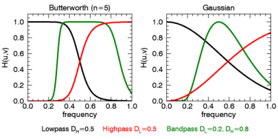
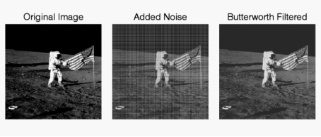
In the following example, we add some sinusoidal noise to an image and filter it with BANDPASS_FILTER, using the BUTTERWORTH keyword.
; Read in the file
File = FILEPATH('moon_landing.png', SUBDIR=['examples','data'])
ImageOriginal = READ PNG(file)
; Generate some sinusoidal noise
XCoords = LINDGEN(300,300) MOD 300
YCoords = TRANSPOSE(xCoords)
Noise = -SIN(xCoords*2)-SIN(yCoords*2)
ImageNoise = imageOriginal + 50*noise
; Filter using a lowpass filter
ImageFiltered = BANDPASS FILTER(imageNoise, 0, 0.4, $
BUTTERWORTH=20)
; Display the original, noise-added, and filtered images
i=IMAGE(imageOriginal, LAYOUT=[3,1,1], TITLE='Original Image', $
DIMENSIONS=[700,300])
i=IMAGE(imageNoise, LAYOUT=[3,1,2], /CURRENT, TITLE='Added Noise')
i=IMAGE(imageFiltered, LAYOUT=[3,1,3], /CURRENT, $
TITLE='Butterworth Filtered')
i.Save, 'bandpass_filter_butterworth_ex.gif', resolution=120
Key takeaway
The BANDPASS_FILTER function applies a lowpass, bandpass, or highpass filter to a one-channel image.
A bandpass filter is useful when the general location of the noise in the frequency domain is known. The bandpass filter allows frequencies within the chosen range through and attenuates frequencies outside of the given range.
Notch filters:
- Are used to remove repetitive "Spectral" noise from an image
- Are like a narrow highpass filter, but they "notch" out frequencies other than the dc component
- Attenuate a selected frequency (and some of its neighbors) and leave other frequencies of the Fourier to transform relatively unchanged
Repetitive noise in an image is sometimes seen as a bright peak somewhere other than the origin. You can suppress such noise effectively by carefully erasing the peaks. One way to do this is to use a notch filter to simply remove that frequency from the picture. This technique is very common in sound signal processing where it is used to remove mechanical or electronic hum, such as the 60Hz hum from AC power. Although it is possible to create notch filters for common noise patterns, in general notch filtering is an ad hoc procedure requiring a human expert to determine what frequencies need to be removed to clean up the signal.
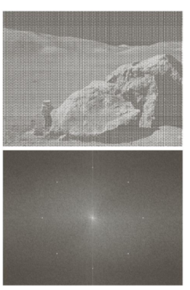
The following is an example of removing synthetic spectral "noise" from an image.
Noisy Image | Fourier Spectrum of Image (noise peaks circled) |
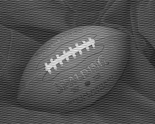 | 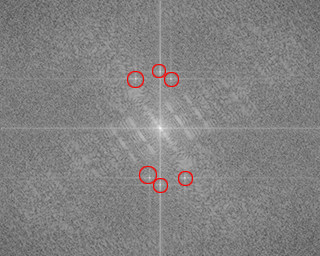 |
Image after Butterworth notch filters | The spectrum of the image after Butterworth notch filters |
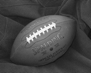 | 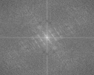 |
The above images were created using four M-files(paddedsize.m, lpfilter.m, dftuv.m, and notch.m), noiseball.png, and the following MATLAB calls
FootBall=imread('noiseball.png');
Imshow(footBall)
%Determine good padding for Fourier transform
PQ = paddedsize(size(footBall));
%Create Notch filters corresponding to extra peaks in the Fourier transform
H1 = notch('btw', PQ(1), PQ(2), 10, 50, 100);
H2 = notch('btw', PQ(1), PQ(2), 10, 1, 400);
H3 = notch('btw', PQ(1), PQ(2), 10, 620, 100);
H4 = notch('btw', PQ(1), PQ(2), 10, 22, 414);
H5 = notch('btw', PQ(1), PQ(2), 10, 592, 414);
H6 = notch('btw', PQ(1), PQ(2), 10, 1, 114);
% Calculate the discrete Fourier transform of the image
F=fft2(double(footBall),PQ(1),PQ(2));
% Apply the notch filters to the Fourier spectrum of the image
FS_football = F.*H1.*H2.*H3.*H4.*H5.*H6;
% convert the result to the spatial domain.
F_football=real(ifft2(FS_football));
% Crop the image to undo padding
F_football=F_football(1:size(footBall,1), 1:size(footBall,2));
%Display the blurred image
Figure, imshow(F_football,[])
% Display the Fourier Spectrum
% Move the origin of the transform to the center of the frequency rectangle.
Fc=fftshift(F);
Fcf=fftshift(FS_football);
% use abs to compute the magnitude and use log to brighten display
S1=log(1+abs(Fc));
S2=log(1+abs(Fcf));
Figure, imshow(S1,[])
Figure, imshow(S2,[])
Key takeaway
Notch filters:
- Are used to remove repetitive "Spectral" noise from an image
- Are like a narrow highpass filter, but they "notch" out frequencies other than the dc component
- Attenuate a selected frequency (and some of its neighbors) and leave other frequencies of the Fourier to transform relatively unchanged
When several interference components are present or if the interference has broad skirts a simply notch filter may remove too much image information.
One solution is to use an optimum filter that minimizes local variances of the restored estimate.
Such “smoothness” constraints are often found in optimum filter design
 1. Manually place a notch pass filter HNP at each noise spike in the frequency domain. The Fourier transform of the interference noise pattern is
 2. Determine the noise pattern in the spatial domain
 3. Conventional thinking would be to simply eliminate noise by subtracting the periodic noise from the noisy image
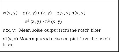
 4. To construct an optimal filter consider
Where w(x,y) is a weighting function.


 5. We use the weighting function w(x,y) to minimize the variance 2(x,y) with respect to w(x,y)
We only need to compute this for one point in each non-overlapping neighborhood.


Key takeaway
When several interference components are present or if the interference has broad skirts a simply notch filter may remove too much image information.
One solution is to use an optimum filter that minimizes local variances of the restored estimate.
Such “smoothness” constraints are often found in optimum filter design
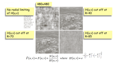
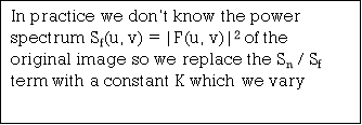
 •If a degraded image is given by degradation + noise
 •Estimate the image by dividing by the degradation function H(u,v)
We can never recover F(u,v) exactly:
1.N(u,v) is not known since (x,y) is a r.v. — estimated
2.If H(u,v) ->0 then the noise term will dominate. Helped by restricting the analysis to (u,v) near the origin.
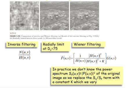
Modeling of Degradation

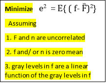

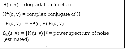
Modeling of Degradation


References:
1. Rafael C. Gonzalez, Richard E. Woods, Digital Image Processing Pearson, Third Edition, 2010
2. Anil K. Jain, Fundamentals of Digital Image Processing Pearson, 2002.
3. Kenneth R. Castleman, Digital Image Processing Pearson, 2006.
4. Rafael C. Gonzalez, Richard E. Woods, Steven Eddins, Digital Image Processing using MATLAB Pearson Education, Inc., 2011.
5. D, E. Dudgeon, and RM. Mersereau, Multidimensional Digital Signal Processing Prentice Hall Professional Technical Reference, 1990.
6. William K. Pratt, Digital Image Processing John Wiley, New York, 2002
7. Milan Sonka et al Image processing, analysis and machine vision Brookes/Cole, Vikas Publishing House, 2nd edition, 1999