Unit – 4
Searching, Sorting and Hashing
Given a collection of objects, the goal of search is to find a particular object in this collection. The objects have key values on which search is performed and data values which correspond to the information one wishes to retrieve once an object is found. For example, a telephone book is a collection of names on which one searches and telephone numbers which correspond to the data being sought. The collection of objects is often stored in a list or an array. Given a collection of objects in an array A[1.. n], the ith element A[i] corresponds to the key value of the ith object in the collection. The input to a search algorithm is an array of objects A, the number of objects n, and the key value being sought x.
Thus Algorithm for Linear Search is
1. start at one end of the list
2. if the current element is not equal to the search target, move to the next element,
3. stop when a match is found or the opposite end of the list is reached.
Function for Linear search is
find(values, target)
{
for( i = 0; i < values.length; i++)
{
if (values[i] == target)
{ return i; }
}
return –1;
}
If element is found this function returns index of that element otherwise it returns –1.
Example : we have an array of integers, like the following:

Let’s search for the number 7. According to function for linear search index for element 7 should be returned. We start at the beginning and check the first element in the array.
9 | 6 | 7 | 12 | 1 | 5 |
First element is 9.Match is not found and hence we move to next element i.e 6.
9 | 6 | 7 | 12 | 1 | 5 |
Again match is not found so move to next element i.e.7.
9 | 6 | 7 | 12 | 1 | 5 |
0 | 1 | 2 | 3 | 4 | 5 |
We found the match at the index position 2. Hence output is 2.
If we try to find element 10 in above array, it will return –1,as 10 is not present in the array.
Complexity Analysis of Linear Search:
Let us assume element x is to be searched in array A of size n.
An algorithm can be analyzed using following three cases.
1. Worst case
2. Average case
3. Best case
1. Worst case : In Linear search worst case happens when element to be searched is not present. When x is not present, the linear search function compares it with all the elements of A one by one. The size of A is n and hence x is to be compared with all n elements. Thus, the worst case time complexity of linear search would be O(n).
2. Average case : In average case analysis, we take all possible inputs and calculate computing time for all of the inputs. Sum all the calculated values and divide the sum by total number of inputs. Following is the value of average case time complexity.
Average Case Time = =
= O (n)
3. Best Case : In linear search , the best case occurs when x is present at the first location. So time complexity in the best case would be O(1).
P1 : Program for Linear Search
#include<stdio.h>
#include<conio.h>
int search(int [],int, int);
void main()
{
int a[20],k,i,n,m;
clrscr();
printf(“\n\n ENTER THE SIZE OF ARRAY”);
scanf(“%d”,&n);
printf(“\n\nENTER THE ARRAY ELEMENTS\n\n”);
for(i=0;i<n;i++)
{
scanf(“%d”,&a[i]);
}
printf(“\n\nENTER THE ELEMENT FOR SEARCH\n”);
scanf(“%d”,&k);
m=search(a,n,k);
if(m==–1)
{
printf(“\n\nELEMENT IS NOT FOUND IN LIST”);
}
else
{
printf(“\n\nELEMENT IS FOUND AT LOCATION %d”,m);
}
}
getch();
}
int search(int a[],int n,int k)
{
int i;
for(i=0;i<n;i++)
{
if(a[i]==k)
{
return i;
}
}
if(i==n)
{
return –1;
}
}
Merits :
1. Simple and easy to implement
2. It works well even on unsorted arrays.
3. It is memory efficient as it does not require copying and partitioning of the array being searched.
Demerits :
Binary search
Binary Search requires sorted array.
Steps to perform binary search on sorted array A of size n are as follows.
1. Initialize lower and upper limit of array to be searched Low=0,High= n–1.
2. Find the middle position
Mid=(Low + High)/2
3. Compare the input key value with the key value of the middle element of the array. It has 3 possibilities.
Case 1 : If keys match then return mid and print element found.
if(key==A[mid])
return mid
Case 2 : If key is less than middle element then element is present in left half of array. Update High and goto step 2.
if(key<A[mid])
High= Mid–1
goto step 2
Case 3 : If key is greater than middle element then element is present in right half of array. Update Low and goto step 2.
if(key>A[mid])
Low= Mid+1
goto step 2
Case 4: if(Low>High)
Print element not found.
Iterative algorithm for Binary Search
int BinarySearch( int A[],int x)
{
int mid,n;
int Low = 0;
int High = n–1;
while ( Low <= High )
{
mid = (Low + High) / 2;
if ( A[mid] == x )
return mid;
if ( A[mid] > x )
High = mid – 1;
else Low = mid + 1;
}
return –1;
}
Example 1 : Let array A= {–1, 5, 6, 18, 19, 25, 46, 78, 102, 114}. We want to find element ‘6’ using binary search.

Solution:
Step 1 : Low=0, High= 9
Step 2 : Mid=(Low + High)/2
Mid = (0+9)/2 =4.5 i.e 4. It means middle element is located at position 4. So A[Mid] is 19.Thus
Low=0
Mid=4
High=9

Step 3 : Compare 6 with 19. It satisfies case 2 of step 3. so High= 4–1=3 and element is present in left half of array. We can ignore right half of array.
Repeat step 2. So mid= (0+3)/2 = 1.5 i.e 1. mid is at position 1. Element 5 is present at position 1.
Low = 0
Mid = 1
High = 3

Again compare 5 with 6. It satisfies case 3 of step 3. so
Low = 1+1=2.
Repeat step 2. Mid= (2+ 3)/2= 2.5 i.e 2 .Mid is at position 2. Element 6 is at position 2.
Low=2
Mid=2
High=3

Compare 6 with 6.
Match is found. Return the position and print element found.
Example 2 : Find 103 in {–1, 5, 6, 18, 19, 25, 46, 78, 102, 114} using Binary Search.

Step 1 : Low=0
High=9
Step 2 : Mid=(0+9)/2=4
So middle element is 19.
Step 3 : Compare(103,19)
103>19 hence element is located at right half of array and we can ignore left half of array. Update Low and recalculate mid.

Middle element is 102. Compare(103,102)
103>102. Recalculate Low and Mid.
Low = 8+1=9
High = 9
Here Low=High and match is not found hence we conclude that element is not present in array.
Example 3 : Find 44 in A={5,12,17,23,38,44,77,84,90} using binary search.
Step 1: Low=0
High=8
Mid=(0+8)/2=4

Middle element is 38. Compare(44,38)
44>38.Thus element is located at right half of array and we can ignore left half of array. Recalculate Low and Mid.
 Middle element is 44. Compare(44,44)
Match is Found. Return index and print “Element Found.”
Algorithm for Recursive Binary Search
int BinarySearch (int A[], int x, int Low, int High)
{
if (High > Low)
return –1;
int mid = (High + Low) / 2;
if (A[mid] == x)
return mid;
if (A[mid] < x)
return BinarySearch(A, x, mid+1, High);
return BinarySearch(A, x, Low, mid–1);
}
P2 : Program for Binary Search
#include<stdio.h>
#include<conio.h>
void main()
{
int n,i,search,f=0,low,high,mid,a[20];
clrscr();
printf("Enter the number of elements:");
scanf("%d",&n);
for(i=1;i<=n;i++)
{
printf("Enter the number in ascending order a[%d]=",i);
scanf("%d",&a[i]);
}
printf("Enter the element to be searched:");
scanf("%d",&search);
low=0;
high=n–1;
while(low<=high)
{
mid=(low+high)/2;
if(search<a[mid])
{
high=mid–1;
}
else if(search>a[mid])
{
low=mid+1;
}
else
{
f=1;
printf("Element is found at the position %d:",mid);
exit();
}
}
if(f==0)
{
printf("Element not found");
}
getch();
}
Complexity Analysis of Binary Search :
Assume our array size is 16.
When n= 16 BinarySearch is called to reduce size to n=8.
When n= 8 BinarySearch is called to reduce size to n=4.
When n= 4 BinarySearch is called to reduce size to n=2.
When n= 2 BinarySearch is called to reduce size to n=1 .
Thus we see that BinarySearch function is called 4 times
i.e. 4 elements of the array were examined for n =16.
Note that 16 = 24
Let us consider a more general case where
n is still a power of 2. Let us say n =2k
After k searches, the while loop is executed k times and n reduces to size 1. Let us assume that each run of the while loop involves at most 4 operations.
Thus total number of operations: 4k.
The value of k can be determined from the expression
2k = n
Taking log of both sides
k = log n
Thus total number of operations = 4 log n.
We conclude that the time complexity of the Binary search method is O(log n), which is much more efficient than the Linear Search method.
Merits :
Binary Search is fast and efficient.
Suitable for large number of values.
Demerits :
Binary search works only on sorted array or list.
Assume we want to sort list in ascending order. Selection sort finds the smallest element from unsorted list and swap it with the element in first position. Then it finds second smallest element and swap it with element at second position. This process is repeated till entire list is sorted in ascending order. Each time we swap elements, we say that we have completed a sort pass. A list of n elements requires n–1 passes to completely rearrange the data.
Procedure for every pass is as follows.
Pass 1 : Find the position P of the smallest in the list of N elements A[l], A[2], . . . , A[N], and then interchange A[P] and A[1] . Then A[1] is sorted.
Pass 2 : Find the position P of the smallest in the sublist of N –1 elements A[2], A[3],. . . , A[N], and then interchange A[P]and A[2]. Then A[l], A[2] is sorted.
Pass 3 : Find the position P of the smallest in the sublist of N–2 elements A[3], A[4], . . . , A[N], and then interchange A[P] and A[3]. Then: A[l], A[2] , A[3] is sorted.
Pass N –1 : Find the position P of the smaller of the elements A[N –1), A[N], and then interchange A[P] and A[N–1]. Then: A[l], A[2], . . . , A[N] is sorted. Thus A is sorted after N –1 passes.
Example 1 :
25 | 79 | 41 | 9 | 34 | 60 |
Fig. 4.2 : Original List
We will apply selection sort on this list.
Pass 1 :

Here smallest element is 9 and 25 is located at first position. so we swap 9 with 25.
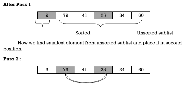
Unsorted sublist has 25 as a smallest element and 79 is located at second position. Hence we swap 25 and 79.
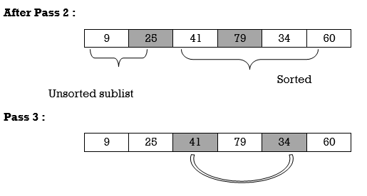
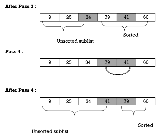
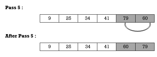
Thus list is sorted.
We will see one more example.
Apply selection sort on array A= {77,30,40,10,88,20,65,56}

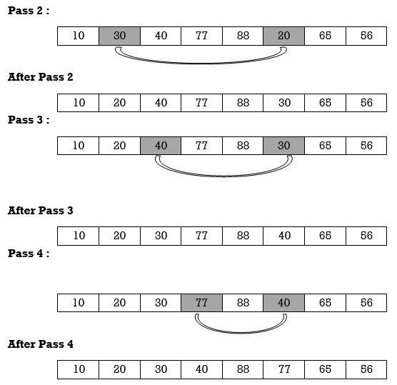
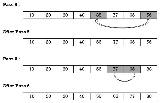
Hence the list is sorted in ascending order by applying selection sort.
Function for Selection Sort
void selectionSort(int A[], int n)
{
int i, j, s, temp;
for (i= 0; i <= n; i ++)
{
s = i;
for (j=i+1; j <= n; j++)
if(A[j] < A[s])
s= j;
// Smallest selected; swap with current element
temp = A[i];
A[i] = A[s];
A[s] = temp;
}
P4 : Program to perform Selection Sort.
#include <stdio.h>
int main()
{
int A[100], n, i, j, s, temp;
/* n=total no. of elements in array
s= smallest element in unsorted array
temp is used for swapping */
printf("Enter number of elements\n");
scanf("%d", &n);
printf("Enter %d integers\n", n);
for ( i = 0 ; i < n ; i++ )
scanf("%d", &A[i]);
for ( i = 0 ; i < ( n – 1 ) ; i++ )
{
s = i;
for ( j = i + 1 ; j < n ; j++ )
{
if ( A[s] > A[j] )
s = j;
}
if ( s != i )
{
temp = A[i];
A[i] = A[s];
A[s] = temp;
}
}
printf("Sorted list in ascending order:\n");
for ( i = 0 ; i < n ; i++ )
printf("%d\n", A[i]);
return 0;
}
Output:
Enter number of elements
5
Enter 5 integers
4
1
7
5
9
Sorted list in ascending order
1
4
5
7
9
Complexity of Selection Sort :
In selection sort outer for loop is executed n–1 times. On the kth time through the outer loop, initially the sorted list holds
k–1 elements and unsorted portion holds n–k+1 elements. In inner for loop 2 elements are compared each time.
Thus, 2*(n–k) elements are examined by the inner loop during the k th pass through the outer loop. But k ranges from 1 to n–1.
Total number of elements examined is:
T(n) = 2*(n –1) + 2*(n–2) + 2*(n–3) + .. + 2*(n–(n–2))
+ 2*(n–(n–1))
= 2*((n–1) + (n–2) + (n–3) + ... + 2 + 1)
(or 2*(sum of first n–1 integers)
= 2*((n–1)*n)/2)
= n2 – n, so complexity of algorithm is O(n2).
Steps to perform Bubble sort are as follows.
Assume we want to sort the elements in ascending order and no two elements are equal.
1. Compare first element with second element. If first element is greater than next element, we interchange their position accordingly. i.e first element is moved to second element’s position and second element is moved to first element’s position. If No, then we don’t interchange any elements.
2. The element in second position is compared with element in third position and the process of interchanging elements is performed if second is greater than third element. The whole process of comparing and interchanging is repeated till last element. When the process gets completed, the largest element in array will get placed in the last position of the array.
Let us consider array A of size n. Then Algorithm for Bubble sort is
1. Set i to 0.
2. Set j to 0.
3. if(A[j]>A[j+1])
swap A[j],A[j+1]
4. Increment j
5. if j<(n–1–i) goto step 3
6. Increment i
7. if(i<n–1) goto step 2.
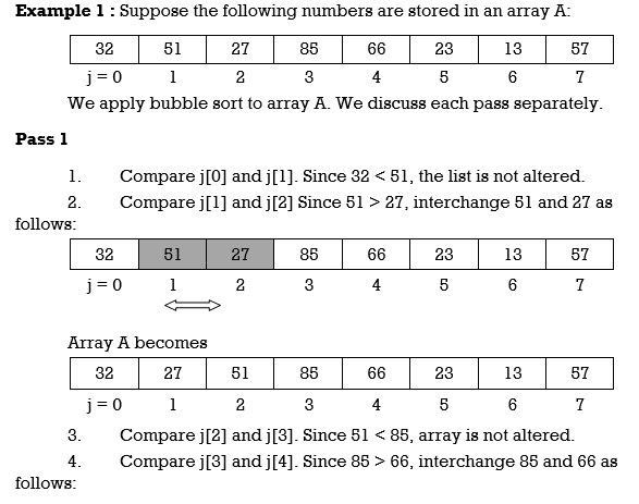

 At the end of this first pass, the largest number, 85, has moved to the last position. However, the rest of the numbers are not sorted, even though some of them have changed their positions.
Pass 2 will move second last number at second last position, Pass 3 will move third last number at third last position and so on. Here we show array after every pass.
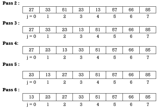 Hence the array is sorted in 6 passes.
We will see one more example
Example 2 : Apply Bubble Sort on array A= {5,3,1,9,8,2,4,7}.
j =0 | 5 | 3 | 1 | 9 | 8 | 2 | 4 | 7 |
j =1 | 3 | 5 | 1 | 9 | 8 | 2 | 4 | 7 |
j =2 | 3 | 1 | 5 | 9 | 8 | 2 | 4 | 7 |
j =3 | 3 | 1 | 5 | 9 | 8 | 2 | 4 | 7 |
j =4 | 3 | 1 | 5 | 8 | 9 | 2 | 4 | 7 |
j =5 | 3 | 1 | 5 | 8 | 2 | 9 | 4 | 7 |
j =6 | 3 | 1 | 5 | 8 | 2 | 4 | 9 | 7 |
j =7 | 3 | 1 | 5 | 8 | 2 | 4 | 7 | 9 |
Pass 2 : i=2
3 | 1 | 5 | 8 | 2 | 4 | 7 | 9 |
1 | 3 | 5 | 8 | 2 | 4 | 7 | 9 |
1 | 3 | 5 | 8 | 2 | 4 | 7 | 9 |
1 | 3 | 5 | 8 | 2 | 4 | 7 | 9 |
1 | 3 | 5 | 2 | 8 | 4 | 7 | 9 |
1 | 3 | 5 | 2 | 4 | 8 | 7 | 9 |
1 | 3 | 5 | 2 | 4 | 7 | 8 | 9 |
Pass 3 :
1 | 3 | 5 | 2 | 4 | 7 | 8 | 9 |
1 | 3 | 5 | 2 | 4 | 7 | 8 | 9 |
1 | 3 | 5 | 2 | 4 | 7 | 8 | 9 |
1 | 3 | 2 | 5 | 4 | 7 | 8 | 9 |
1 | 3 | 2 | 4 | 5 | 7 | 8 | 9 |
Pass 4 :
1 | 3 | 2 | 4 | 5 | 7 | 8 | 9 |
1 | 3 | 2 | 4 | 5 | 7 | 8 | 9 |
1 | 2 | 3 | 4 | 5 | 7 | 8 | 9 |
This array gets sorted in 4 passes only.
Example : Apply Bubble Sort on array A= {23,78,45,8,32,56}
Pass 1 :
23 | 78 | 45 | 8 | 32 | 56 |
23 | 78 | 45 | 8 | 32 | 56 |
23 | 45 | 78 | 8 | 32 | 56 |
23 | 45 | 8 | 78 | 32 | 56 |
23 | 45 | 8 | 32 | 78 | 56 |
23 | 45 | 8 | 32 | 56 | 78 |
Pass 2 :
23 | 45 | 8 | 32 | 56 | 78 |
23 | 45 | 8 | 32 | 56 | 78 |
23 | 8 | 45 | 32 | 56 | 78 |
23 | 8 | 32 | 45 | 56 | 78 |
Pass 3 :
23 | 8 | 32 | 45 | 56 | 78 |
8 | 23 | 32 | 45 | 56 | 78 |
This array is sorted in 3 passes.
P3: Write a Program for Bubble sort in C
#include <stdio.h>
#include<conio.h>
void bubble_sort(int A[], int n);
int main()
{
int A[100], n, i, j, swap;
printf("Enter number of elements\n");
scanf("%d", &n);
printf("Enter the elements\n", );
for (i = 0; i < n; i++)
scanf("%d", &A[i]);
bubble_sort(A, n);
printf("Sorted list in ascending order:\n");
for ( i = 0 ; i < n ; i++ )
printf("%ld\n", A[i]);
return 0;
}
void bubble_sort(int A[], int n)
{
int i, j, t;
for (i = 0 ; i < ( n – 1 ); i++)
{
for (j = 0 ; j < (n – i – 1); j++)
{
if (A[j] > list[j+1])
{
/* Swapping */
t = A[j];
A[j] = A[j+1];
A[j+1] = t;
}
}
}
}
Complexity Bubble sort:
Suppose we have a list with n elements, and each element perform n – 1 comparisons with elements to its left, and swap, if necessary.
Best Case: If the list is already sorted, only one iteration is performed and complexity is O(1).
Average and Worst case: For n elements at most n – 1 swap operations is performed in each pass. The worst and average case complexity is O(n2).
Insertion Sort reads all elements from 1 to n and inserts each element at its proper position. This sorting method works well on small list of elements.
Procedure for each pass is as follows.
Pass 1 :
A[l] by itself is trivially sorted.
Pass 2 :
A[2] is inserted either before or after A[l] so that: A[l], A[2] is sorted.
Pass 3 :
A[3] is inserted into its proper place so that: A[l], A[2], A[3] is sorted.
Pass 4 :
A[4] is inserted into its proper place A[l], A[2], A[3], A[4] is sorted.
Pass N :
A[N] is inserted into its proper place in so that:
A[l], A[ 2 ] , . . . , A[ N ] is sorted
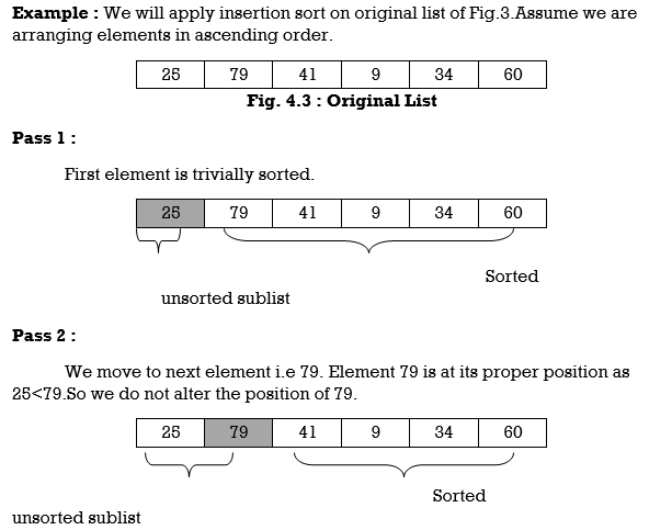
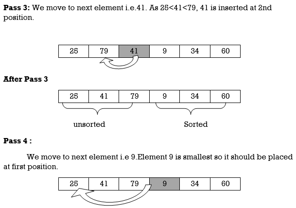
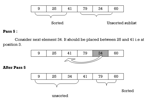
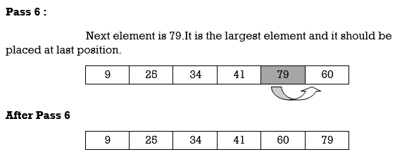
Hence the list is sorted using insertion sort.
We will see one more example.
Apply Insertion sort on array A= {77,30,40,10,88,20,65,56}
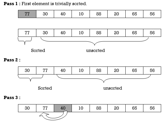
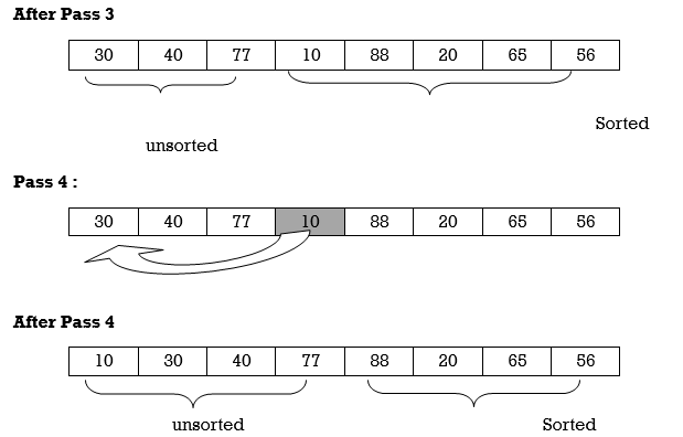

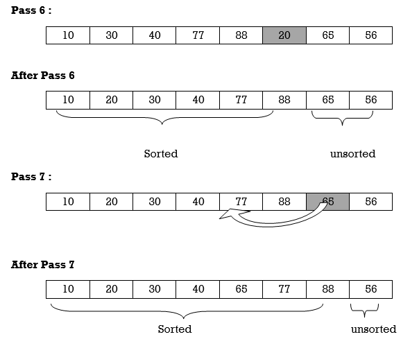
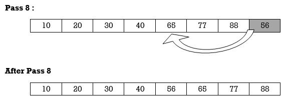
Hence the list is sorted using Insertion sort.
C Function for Insertion Sort
void insertionSort(int A[], int n)
{
int i, p, temp, j;
for (i = 1; i<=n; i++)
{
p= 0;
temp = A[i];
for (j=i–1; j >= 0 && !p;)
if(temp < A[j])
{
A[j + 1]= A[j];
j––;
}
else
p = 1;
A[j + 1] = temp;
}
return;
}
P5 : Program to implement insertion sort.
#include <stdio.h>
int main()
{
int n, A[100], i, j, t;
printf("Enter number of elements\n");
scanf("%d", &n);
printf("Enter %d integers\n", n);
for (i = 0; i < n; i++) {
scanf("%d", &A[i]);
}
for (i = 1 ; i <=( n – 1); i++)
{
j = i;
while ( j > 0 && A[j] < A[j–1])
{
t = A[j];
A[j] = A[j–1];
A[j–1] = t;
j––;
}
}
printf("Sorted list in ascending order:\n");
for (i = 0; i <= n – 1; i++) {
printf("%d\n", A[i]);
}
return 0;
}
Output :
Enter number of elements
5
Enter 5 integers
9
4
2
5
3
Sorted list in ascending order
2
3
4
5
9
Complexity of Insertion Sort :
Worst Case Complexity: In the worst case, for each i we do (i – 1) swaps inside the inner for–loop–therefore, overall number of swaps (when i goes from 2 to n in the outer for loop) is
T(n) = 1 + 2 + 3 +...+(I – 1) +....+ n – 1
= n (n – 1)/2
= O(n2)
Average case Complexity is O(n2).
Best Case Complexity is O(n).
Quick sort is most efficient method of sorting .It uses divide and conquer strategy to sort the elements. In quicksort, we divide the array of items to be sorted into two partitions and then call the quicksort procedure recursively to sort the two partitions. For this we choose a pivot element and arrange all elements such that all the elements in the left part are less than the pivot and all those in the right part are greater than it.
Algorithm to implement Quick Sort is as follows.
Consider array A of size n to be sorted. p is pivot element. Index positions of first and last element of array A is denoted by ‘first’ and ‘last’.
C function for Quick sort
x=0,y=n–1
void Quicksort(A,x,y)
{
if(x<y)
{
first=x;
last=y;
p=A[x];
while(first<last)
{
while(A[first]<p)
first++;
while(A[last]>p)
last ––;
if(first<last)
swap(A[first],A[last])
}
swap(A[x],A[y])
Quicksort(A,x,last–1);
Quicksort(A,first+1,y);
}
We will see examples on Quick sort
Example : Apply Quicksort on array
A= {27,6,39,2,65,12,57,18,49,19}
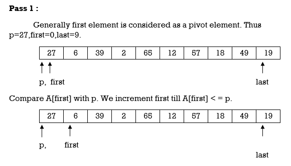
Now, compare A[last] with p. We decrement last till A[last]>=p.
Here 19 < 27. So condition A[last]>=p becomes false and we stop decrementing last.
Currently first=2 and last=9.
i.e first < last so we swap A[first] and A[last].Swapping 39 and 19 we get
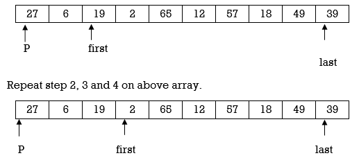
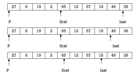 Here again first<last so we swap A[first] and A[last]. Swapping 65 and 18 we get
Repeat step 2,3 and 4.
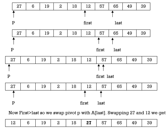 Here we complete Pass 1.Now pivot element is 27 and it divides array in left and right partition. We can see that elements less than pivot are in left partition and elements greater than pivot are in right partition.
Now we continue same procedure for left and right partition. Here we see results of corresponding passes.
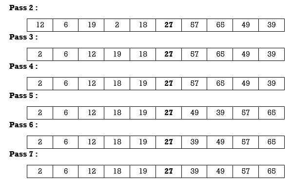 We will see another example.
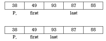
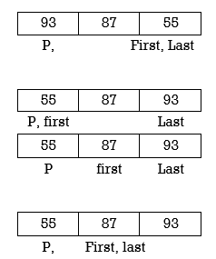
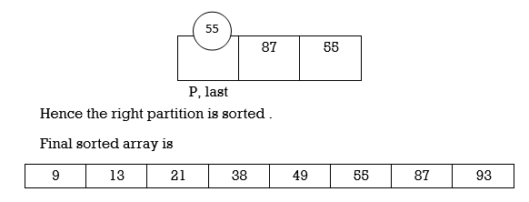
Example : Apply Quicksort on array A={21,55,49,38,13,93,87,9}
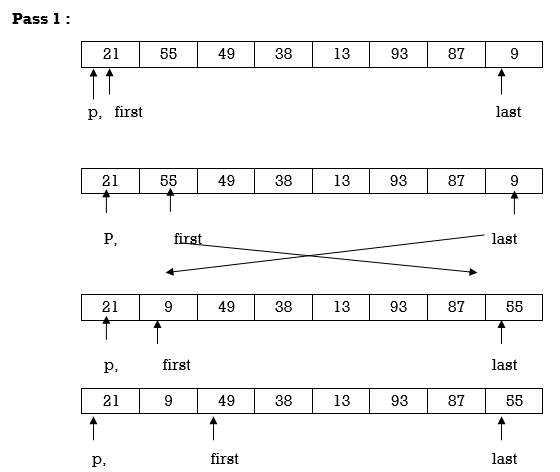

Now first>last hence swap pivot and A[last].Swapping 21 and 13 we get
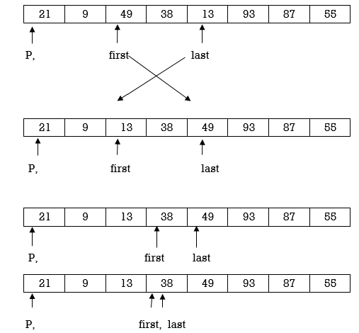
Now first > last hence swap pivot and A [last]’. Swapping 21 and 13 we get
 Left Partition
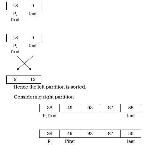

Example : Apply Quick Sort on A={42,15,9,75,18,2,55,1,64}
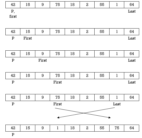
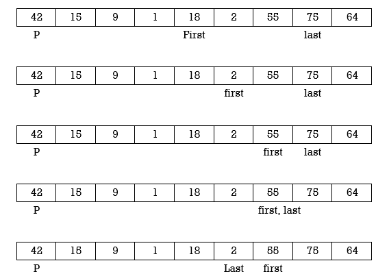
Swap p and A[last]
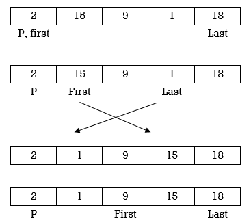
 Applying Quick sort on left partition
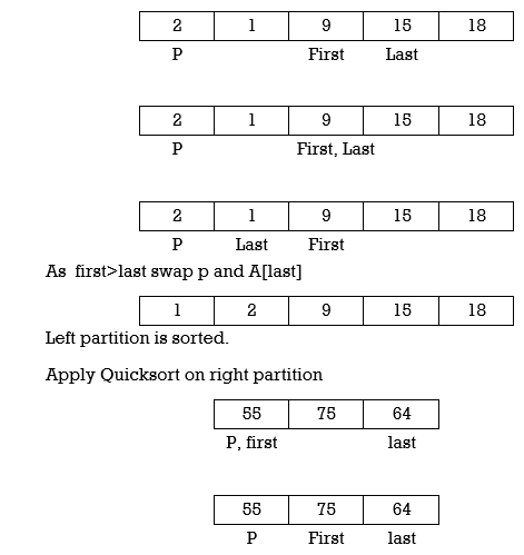


Program for Quick Sort:
#include<stdio.h>
void quicksort(int A[10],int,int);
int main(){
int A[20],n,i;
printf("Enter size of the array: ");
scanf("%d",&n);
printf("Enter %d elements: ",n);
for(i=0;i<n;i++)
scanf("%d",&A[i]);
quicksort(A,0,n–1);
printf("Sorted elements: ");
for(i=0;i<n;i++)
printf(" %d",A[i]);
return 0;
}
void quicksort(int A[20],int first, int last)
{
int pivot,j,temp,i;
if(first<last){
pivot=first;
i=first;
j=last;
while(i<j){
while(A[i]<=A[pivot]&&i<last)
i++;
while(A[j]>A[pivot])
j––;
if(i<j){
temp=A[i];
A[i]=A[j];
A[j]=temp;
}
}
temp=A[pivot];
A[pivot]=A[j];
A[j]=temp;
quicksort(A,first,j–1);
quicksort(A,j+1,last);
}
}
Output :
Enter size of the array: 5
Enter 5 elements: 3 8 0 1 2
Sorted elements: 0 1 2 3 8
Complexity of Quick Sort
The time to sort the file is equal to
Worst case analysis
The pivot is the smallest element
T(N) = T(N – 1) + cN, N > 1
T(N – 1) = T(N – 2) + c(N – 1)
T(N – 2) = T(N – 3) + c(N – 2)
T(N – 3) = T(N – 4) + c(N– 3)
T(2) = T(1) + c.2
Add all equations:
T(N) + T(N – 1) + T(N – 2) + … + T(2) =
= T(N – 1) + T(N – 2) + … + T(2) + T(1) + c(N) + c(N – 1) + c(N – 2) + … + c.2
T(N) = T(1) + c times (the sum of 2 thru N) = T(1) + c(N(N+1)/2 –1) = O(N2)
Best–case analysis:
The pivot is in the middle
T(N) = 2T(N/2) + cN
Divide by N:
T(N) / N = T(N/2) / (N/2) + c
T(N/2) / (N/2) = T(N/4) / (N/4) + c
T(N/4) / (N/4) = T(N/8) / (N/8) + c
…..
T(2) / 2 = T(1) / (1) + c
Add all equations:
T(N) / N + T(N/2) / (N/2) + T(N/4) / (N/4) + …. + T(2) / 2
= (N/2) / (N/2) + T(N/4) / (N/4) + … + T(1) / (1) + c.logN
After crossing the equal terms:
T(N)/N = T(1) + cLogN
T(N) = N + NcLogN = O(NlogN)
Average case analysis
Similar computations, resulting in T(N) = O(NlogN)
The average value of T(i) is 1/N times the sum of T(0) through T(N–1)
1/N S T(j), j = 0 thru N–1
T(N) = 2/N (S T(j)) + cN
Multiply by N
NT(N) = 2(S T(j)) + cN*N
To remove the summation, we rewrite the equation for N–1:
(N–1)T(N–1) = 2(S T(j)) + c(N–1)2, j = 0 thru N–2
and subtract:
NT(N) – (N–1)T(N–1) = 2T(N–1) + 2cN –c
NT(N) = (N+1)T(N–1) + 2cN
Divide by N(N+1):
T(N)/(N+1) = T(N–1)/N + 2c/(N+1)
T(N)/(N+1) = T(N–1)/N + 2c/(N+1)
T(N–1)/(N) = T(N–2)/(N–1)+ 2c/(N)
T(N–2)/(N–1) = T(N–3)/(N–2) + 2c/(N–1)
….
T(2)/3 = T(1)/2 + 2c /3
Add the equations and cross equal terms:
T(N)/(N+1) = T(1)/2 +2c S (1/j), j = 3 to N+1
The sum S (1/j), j =3 to N–1, is about LogN
Thus T(N) = O(NlogN)
Merge Sort is based on divide and conquer strategy. It divides the unsorted list into n sublists such that each sublist contains one element. Each sublist is then sorted and merged until there is only one sublist.
Step 1 : Divide the list into sublists such that each sublist contains only one element.
Step 2 : Sort each sublist and Merge them.
Step 3 : Repeat Step 2 till the entire list is sorted.
Example : Apply Merge Sort on array A= {85,24,63,45,17,31,96,50}
Step1 : A contains 8 elements. First we divide the list into two sublists such that each sublist contains 4 elements. Then we divide each sublist of 4 elements into sublist of two elements each. Finally every sublist contains only one element.

Fig.
Step 2 : Now we start from bottom. Compare 1st and 2nd element. Sort and merge them. Apply this for all bottom elements.
Thus we got 4 sublists as follows
24 | 85 |
| 45 | 63 |
| 17 | 31 |
| 50 | 96 |
Step 3 : Repeat this sorting and merging until entire list is sorted. Thus above four sublists are sorted and merged to form 2 sublists.
24 | 85 | 63 | 85 |
| 17 | 31 | 50 | 96 |
Finally above 2 sublists are again sorted and merged in one sublist.
17 | 24 | 31 | 45 | 50 | 63 | 85 | 96 |
We will see one more example on merge sort.
Example : Apply merge Sort on array A={10,5,7,6,1,4,8,3,2,9,12,11}
Step 1 :

Fig.
Algorithm for Merge Sort:
Let x = no. of elements in array A
y = no. of elements in array B
C = sorted array with no. of elements n
n = x+y
Following algorithm merges a sorted x element array A and sorted y element array B into a sorted array C, with n = x + y elements. We must always keep track of the locations of the smallest element of A and the smallest element of B which have not yet been placed in C. Let LA and LB denote these locations, respectively. Also, let LC denote the location in C to be filled. Thus, initially, we set
LA : = 1,
LB : = 1 and
LC : = 1.
At each step , we compare A[LA] and B[LB] and assign the smaller element to C[LC].
Then
LC:= LC + 1,
LA: = LA + 1, if new element has come from A .
LB: = LB + 1, if new element has come from B.
Furthermore, if LA> x, then the remaining elements of B are assigned to C;
 LB >y, then the remaining elements of A are assigned to C.
Thus the algorithm becomes
MERGING ( A, x, B, y, C)
1. [Initialize ] Set LA : = 1 , LB := 1 AND LC : = 1
2. [Compare] Repeat while LA <= x and LB <= y
If A[LA] < B[LB] , then
(a) [Assign element from A to C ] set C[LC] = A[LA]
(b) [Update pointers ] Set LC := LC +1 and LA = LA+1
Else
(a) [Assign element from B to C] Set C[LC] = B[LB]
(b) [Update Pointers] Set LC := LC +1 and LB = LB +1
[End of loop]
3. [Assign remaining elements to C]
If LA > x , then
Repeat for K= 0 ,1,2,........,y–LB
Set C[LC+K] = B[LB+K]
[End of loop]
Else
Repeat for K = 0,1,2,......,x–LA
Set C[LC+K] = A[LA+K]
[End of loop]
4. Exit
Program for Merge Sort
#include<stdio.h>
#define MAX 50
void mergeSort(int A[],int first,int mid,int high);
void divide(int A[],int first,int last);
int main(){
int merge[MAX],i,n;
printf("Enter the total number of elements: ");
scanf("%d",&n);
printf("Enter the elements which to be sort: ");
for(i=0;i<n;i++){
scanf("%d",&merge[i]);
}
divide(merge,0,n–1);
printf("After merge sorting elements are: ");
for(i=0;i<n;i++){
printf("%d ",merge[i]);
}
return 0;
}
void divide(int A[],int first, int last)
{
int mid;
if(first<last){
mid=(first+last)/2;
divide(A,first,mid);
divide(A,mid+1,last);
mergeSort(A,first,mid,last);
}
}
void mergeSort(int A[],int first,int mid,int last)
{
int i,m,k,l,temp[MAX];
l=first;
i=first;
m=mid+1;
while((l<=mid)&&(m<=last)){
if(A[l]<=A[m]){
temp[i]=A[l];
l++;
}
else{
temp[i]=A[m];
m++;
}
i++;
}
if(l>mid){
for(k=m;k<=last;k++){
temp[i]=arr[k];
i++;
}
}
else{
for(k=l;k<=mid;k++){
temp[i]=arr[k];
i++;
}
}
for(k=first;k<=last;k++){
A[k]=temp[k];
}
}
Output :
Enter the total number of elements: 5
Enter the elements which to be sort: 3 1 6 4 7
After merge sorting elements are: 1 3 4 6 7
Complexity of Merge Sort :
Time to mergesort N elements = Time to mergesort N/2 elements plus time to merge two arrays each N/2 elements.
Time to merge two arrays each N/2 elements is linear, i.e. N
Thus we have:
(1) T(1) = 1
(2) T(N) = 2T(N/2) + N
Dividing (2) by N we get:
(3) T(N) / N = T(N/2) / (N/2) + 1
N is a power of two, so we can write
(4) T(N/2) / (N/2) = T(N/4) / (N/4) +1
(5) T(N/4) / (N/4) = T(N/8) / (N/8) +1
(6) T(N/8) / (N/8) = T(N/16) / (N/16) +1
(7) ……
(8) T(2) / 2 = T(1) / 1 + 1
Adding equations (3) through (8), the sum of their left–hand sides will be equal to the sum of their right–hand sides:
T(N) / N + T(N/2) / (N/2) + T(N/4) / (N/4) + … + T(2)/2
= T(N/2) / (N/2) + T(N/4) / (N/4) + ….+ T(2) / 2 + T(1) / 1 + LogN
(LogN is the sum of 1s in the right–hand sides)
After crossing the equal term, we get
(9) T(N)/N = T(1)/1 + LogN
T(1) is 1, hence we obtain
(10) T(N) = N + NlogN = O(NlogN)
Hence the complexity of the MergeSort algorithm is O(NlogN).
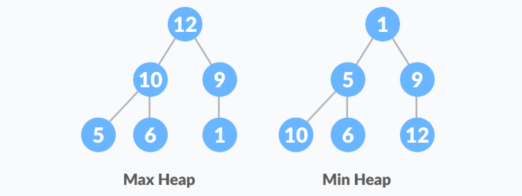
Heap is a special tree-based data structure. A binary tree is said to follow a heap data structure if it is a complete binary tree
All nodes in the tree follow the property that they are greater than their children i.e. the largest element is at the root and both its children and smaller than the root and so on. Such a heap is called a max-heap. If instead, all nodes are smaller than their children, it is called a min-heap
The following example diagram shows Max-Heap and Min-Heap.

Starting from a complete binary tree, we can modify it to become a Max-Heap by running a function called heapify on all the non-leaf elements of the heap.
heapify(array)
Root = array[0]
Largest = largest( array[0] , array [2*0 + 1]. array[2*0+2])
if(Root != Largest)
Swap(Root, Largest)
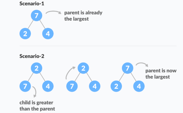
The example above shows two scenarios - one in which the root is the largest element and we don't need to do anything. And another in which the root had a larger element as a child and we needed to swap to maintain max-heap property.
In comparison based sorting, elements of an array are compared with each other to find the sorted array.
Bubble sort and Insertion sort –
Average and worst case time complexity: n^2
Best case time complexity: n when array is already sorted.
Worst case: when the array is reverse sorted.
Selection sort –
Best, average and worst case time complexity: n^2 which is independent of distribution of data.
Merge sort –
Best, average and worst case time complexity: nlogn which is independent of distribution of data.
Heap sort –
Best, average and worst case time complexity: nlogn which is independent of distribution of data.
Quick sort –
It is a divide and conquer approach with recurrence relation:
T(n) = T(k) + T(n-k-1) + cn
Worst case: when the array is sorted or reverse sorted, the partition algorithm divides the array in two subarrays with 0 and n-1 elements. Therefore,
T(n) = T(0) + T(n-1) + cn
Solving this we get, T(n) = O(n^2)
Best case and Average case: On an average, the partition algorithm divides the array in two subarrays with equal size. Therefore,
T(n) = 2T(n/2) + cn
Solving this we get, T(n) = O(nlogn)
Non-comparison based sorting –
In non-comparison based sorting, elements of array are not compared with each other to find the sorted array.
Radix sort –
Best, average and worst case time complexity: nk where k is the maximum number of digits in elements of array.
Count sort –
Best, average and worst case time complexity: n+k where k is the size of count array.
Bucket sort –
Best and average time complexity: n+k where k is the number of buckets.
Worst case time complexity: n^2 if all elements belong to same bucket.
In-place/Outplace technique –
A sorting technique is inplace if it does not use any extra memory to sort the array.
Among the comparison based techniques discussed, only merge sort is outplaced technique as it requires an extra array to merge the sorted subarrays.
Among the non-comparison based techniques discussed, all are outplaced techniques. Counting sort uses a counting array and bucket sort uses a hash table for sorting the array.
Online/Offline technique –
A sorting technique is considered Online if it can accept new data while the procedure is ongoing i.e. complete data is not required to start the sorting operation.
Among the comparison based techniques discussed, only Insertion Sort qualifies for this because of the underlying algorithm it uses i.e. it processes the array (not just elements) from left to right and if new elements are added to the right, it doesn’t impact the ongoing operation.
Stable/Unstable technique –
A sorting technique is stable if it does not change the order of elements with the same value.
Out of comparison based techniques, bubble sort, insertion sort and merge sort are stable techniques. Selection sort is unstable as it may change the order of elements with the same value. For example, consider the array 4, 4, 1, 3.
In the first iteration, the minimum element found is 1 and it is swapped with 4 at 0th position. Therefore, the order of 4 with respect to 4 at the 1st position will change. Similarly, quick sort and heap sort are also unstable.
Hashing is an important Data Structure which is designed to use a special function called the Hash function which is used to map a given value with a particular key for faster access of elements. The efficiency of mapping depends of the efficiency of the hash function used.
Let a hash function H(x) maps the value  at the index x%10 in an Array. For example if the list of values is [11,12,13,14,15] it will be stored at positions {1,2,3,4,5} in the array or Hash table respectively.
Reference Books
1. Algorithms, Data Structures, and Problem Solving with C++”, Illustrated Edition by Mark Allen Weiss, Addison-Wesley Publishing Company.
2. “How to Solve it by Computer”, 2nd Impression by R.G. Dromey, Pearson Education.
3. “Fundamentals of Data Structures”, Illustrated Edition by Ellis Horowitz, Sartaj Sahni, Computer Science Press.