UNIT-3
Overview of Brute-Force
Algorithm:
An algorithm is a step-by-step procedure to solve a problem. A good algorithm should be optimized in terms of time and space. Different types of problems require different types of algorithmic-techniques to be solved in the most optimized manner. There are many types of algorithms but the most important and the fundamental algorithms that you must know will be discussed in this article.
Brute Force Algorithm:
This is the most basic and simplest type of algorithm. A Brute Force Algorithm is the straightforward approach to a problem i.e., the first approach that comes to our mind on seeing the problem. More technically it is just like iterating every possibility available to solve that problem.
For Example: If there is a lock of 4-digit PIN. The digits to be chosen from 0-9 then the brute force will be trying all possible combinations one by one like 0001, 0002, 0003, 0004, and so on until we get the right PIN. In the worst case, it will take 10,000 tries to find the right combination.
Recursive Algorithm:
This type of algorithm is based on recursion. In recursion, a problem is solved by breaking it into subproblems of the same type and calling own self again and again until the problem is solved with the help of a base condition.
Some common problem that is solved using recursive algorithms are Factorial of a Number, Fibonacci Series, Tower of Hanoi, DFS for Graph, etc.
Divide and Conquer Algorithm:
In Divide and Conquer algorithms, the idea is to solve the problem in two sections, the first section divides the problem into subproblems of the same type. The second section is to solve the smaller problem independently and then add the combined result to produce the final answer to the problem.
Some common problem that is solved using Divide and Conquers Algorithms are Binary Search, Merge Sort, Quick Sort, Strassen’s Matrix Multiplication, etc.
Dynamic Programming Algorithms:
This type of algorithm is also known as the memorization technique because in this the idea is to store the previously calculated result to avoid calculating it again and again. In Dynamic Programming, divide the complex problem into smaller overlapping sub problems and storing the result for future use.
The following problems can be solved using Dynamic Programming algorithm Knapsack Problem, Weighted Job Scheduling, Floyd Warshall Algorithm, Dijkstra Shortest Path Algorithm,etc.
Greedy Algorithm:
In the Greedy Algorithm, the solution is built part by part. The decision to choose the next part is done on the basis that it gives the immediate benefit. It never considers the choices that had taken previously.
Some common problems that can be solved through the Greedy Algorithm are Prim’s Algorithm, Kruskal’s Algorithm, Huffman Coding,etc.
Backtracking Algorithm:
In Backtracking Algorithm, the problem is solved in an incremental way i.e. it is an algorithmic-technique for solving problems recursively by trying to build a solution incrementally, one piece at a time, removing those solutions that fail to satisfy the constraints of the problem at any point of time.
Brute Force Attack
A Brute force attack is a well-known breaking technique, by certain records, brute force attacks represented five percent of affirmed security ruptures. A brute force attack includes ‘speculating’ username and passwords to increase unapproved access to a framework. Brute force is a straightforward attack strategy and has a high achievement rate.
A few attackers use applications and contents as brute force devices. These instruments evaluate various secret word mixes to sidestep confirmation forms. In different cases, attackers attempt to get to web applications via scanning for the correct session ID. Attacker inspiration may incorporate taking data, contaminating destinations with malware, or disturbing help.
While a few attackers still perform brute force attacks physically, today practically all brute force attacks are performed by bots. Attackers have arrangements of usually utilized accreditations, or genuine client qualifications, got through security breaks or the dull web. Bots deliberately attack sites and attempt these arrangements of accreditations, and advise the attacker when they obtain entrance.
Types of Brute Force Attacks:
- Dictionary attacks – surmises usernames or passwords utilizing a dictionary of potential strings or phrases.
- Rainbow table attacks – a rainbow table is a precomputed table for turning around cryptographic hash capacities. It very well may be utilized to figure a capacity up to a specific length comprising of a constrained arrangement of characters.
- Reverse brute force attack – utilizes a typical password or assortment of passwords against numerous conceivable usernames. Focuses on a network of clients for which the attackers have recently acquired information.
- Hybrid brute force attacks – begins from outer rationale to figure out which password variety might be destined to succeed, and afterward proceeds with the simple way to deal with attempt numerous potential varieties.
- Simple brute force attack – utilizes an efficient way to deal with ‘surmise’ that doesn’t depend on outside rationale.
- Credential stuffing – utilizes beforehand known password-username sets, attempting them against numerous sites. Adventures the way that numerous clients have the equivalent username and password across various frameworks.
How to Prevent Brute Force Password Hacking ?
To protect your organization from brute force password hacking, enforce the use of strong passwords.
Passwords should:
- Never use information that can be found online (like names of family members).
- Have as many characters as possible.
- Combine letters, numbers, and symbols.
- Avoid common patterns.
- Be different for each user account.
- Change your password periodically
- Use strong and long password
- Use multifactor authentication
Key takeaway
Brute Force Algorithm:
This is the most basic and simplest type of algorithm. A Brute Force Algorithm is the straightforward approach to a problem i.e., the first approach that comes to our mind on seeing the problem. More technically it is just like iterating every possibility available to solve that problem.
For Example: If there is a lock of 4-digit PIN. The digits to be chosen from 0-9 then the brute force will be trying all possible combinations one by one like 0001, 0002, 0003, 0004, and so on until we get the right PIN. In the worst case, it will take 10,000 tries to find the right combination.
"Greedy Method finds out of many options, but you have to choose the best option."
In this method, we have to find out the best method/option out of many present ways.
In this approach/method we focus on the first stage and decide the output, don't think about the future.
This method may or may not give the best output.
Greedy Algorithm solves problems by making the best choice that seems best at the particular moment. Many optimization problems can be determined using a greedy algorithm. Some issues have no efficient solution, but a greedy algorithm may provide a solution that is close to optimal. A greedy algorithm works if a problem exhibits the following two properties:
- Greedy Choice Property: A globally optimal solution can be reached at by creating a locally optimal solution. In other words, an optimal solution can be obtained by creating "greedy" choices.
- Optimal substructure: Optimal solutions contain optimal subsolutions. In other words, answers to subproblems of an optimal solution are optimal.
- machine scheduling
- Fractional Knapsack Problem
- Minimum Spanning Tree
- Huffman Code
- Job Sequencing
- Activity Selection Problem
Steps for achieving a Greedy Algorithm are:
- Feasible: Here we check whether it satisfies all possible constraints or not, to obtain at least one solution to our problems.
- Local Optimal Choice: In this, the choice should be the optimum which is selected from the currently available
- Unalterable: Once the decision is made, at any subsequence step that option is not altered.
The activity selection problem is a mathematical optimization problem. Our first illustration is the problem of scheduling a resource among several challenge activities. We find a greedy algorithm provides a well designed and simple method for selecting a maximum- size set of manually compatible activities.
Suppose S = {1, 2....n} is the set of n proposed activities. The activities share resources which can be used by only one activity at a time, e.g., Tennis Court, Lecture Hall, etc. Each Activity "i" has start time si and a finish time fi, where si ≤fi. If selected activity "i" take place meanwhile the half-open time interval [si,fi). Activities i and j are compatible if the intervals (si, fi) and [si, fi) do not overlap (i.e. i and j are compatible if si ≥fi or si ≥fi). The activity-selection problem chosen the maximum- size set of mutually consistent activities.
Algorithm Of Greedy- Activity Selector:
GREEDY- ACTIVITY SELECTOR (s, f)
1. n ← length [s]
2. A ← {1}
3. j ← 1.
4. for i ← 2 to n
5. do if si ≥ fi
6. then A ← A ∪ {i}
7. j ← i
8. return A
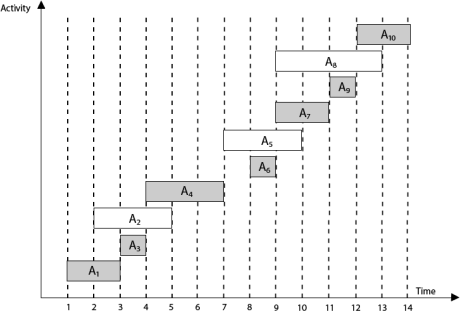
Example: Given 10 activities along with their start and end time as
S = (A1 A2 A3 A4 A5 A6 A7 A8 A9 A10)
Si = (1,2,3,4,7,8,9,9,11,12)
fi = (3,5,4,7,10,9,11,13,12,14)
Compute a schedule where the greatest number of activities takes place.
Solution: The solution to the above Activity scheduling problem using a greedy strategy is illustrated below:
Arranging the activities in increasing order of end time
|
Now, schedule A1
Next schedule A3 as A1 and A3 are non-interfering.
Next skip A2 as it is interfering.
Next, schedule A4 as A1 A3 and A4 are non-interfering, then next, schedule A6 as A1 A3 A4 and A6 are non-interfering.
Skip A5 as it is interfering.
Next, schedule A7 as A1 A3 A4 A6 and A7 are non-interfering.
Next, schedule A9 as A1 A3 A4 A6 A7 and A9 are non-interfering.
Skip A8 as it is interfering.
Next, schedule A10 as A1 A3 A4 A6 A7 A9 and A10 are non-interfering.
Thus the final Activity schedule is:
|
Key takeaway
"Greedy Method finds out of many options, but you have to choose the best option."
In this method, we have to find out the best method/option out of many present ways.
In this approach/method we focus on the first stage and decide the output, don't think about the future.
This method may or may not give the best output.
Dynamic Programming is the most powerful design technique for solving optimization problems.
Divide & Conquer algorithm partition the problem into disjoint subproblems solve the subproblems recursively and then combine their solution to solve the original problems.
Dynamic Programming is used when the subproblems are not independent, e.g. when they share the same subproblems. In this case, divide and conquer may do more work than necessary, because it solves the same sub problem multiple times.
Dynamic Programming solves each subproblems just once and stores the result in a table so that it can be repeatedly retrieved if needed again.
Dynamic Programming is a Bottom-up approach- we solve all possible small problems and then combine to obtain solutions for bigger problems.
Dynamic Programming is a paradigm of algorithm design in which an optimization problem is solved by a combination of achieving sub-problem solutions and appearing to the "principle of optimality".
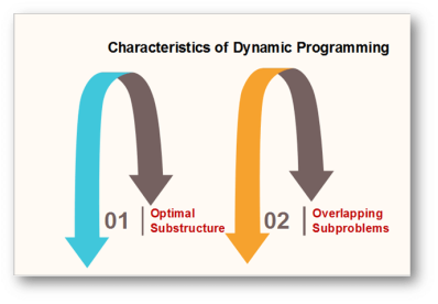
Characteristics of Dynamic Programming:
Dynamic Programming works when a problem has the following features:-
|
Fig 1 - Characteristics of Dynamic Programming
- Optimal Substructure: If an optimal solution contains optimal sub solutions then a problem exhibits optimal substructure.
- Overlapping subproblems: When a recursive algorithm would visit the same subproblems repeatedly, then a problem has overlapping subproblems.
If a problem has optimal substructure, then we can recursively define an optimal solution. If a problem has overlapping subproblems, then we can improve on a recursive implementation by computing each subproblem only once.
If a problem doesn't have optimal substructure, there is no basis for defining a recursive algorithm to find the optimal solutions. If a problem doesn't have overlapping sub problems, we don't have anything to gain by using dynamic programming.
If the space of subproblems is enough (i.e. polynomial in the size of the input), dynamic programming can be much more efficient than recursion.
Elements of Dynamic Programming
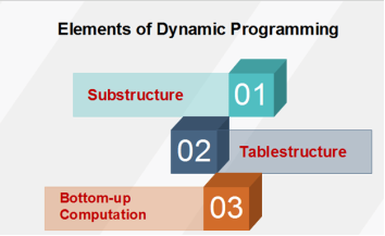
There are basically three elements that characterize a dynamic programming algorithm:-
|
Fig 2 - Elements of Dynamic Programming
- Substructure: Decompose the given problem into smaller subproblems. Express the solution of the original problem in terms of the solution for smaller problems.
- Table Structure: After solving the sub-problems, store the results to the sub problems in a table. This is done because subproblem solutions are reused many times, and we do not want to repeatedly solve the same problem over and over again.
- Bottom-up Computation: Using table, combine the solution of smaller subproblems to solve larger subproblems and eventually arrives at a solution to complete problem.
Note: Bottom-up means:-
- Start with smallest subproblems.
- Combining their solutions obtain the solution to sub-problems of increasing size.
- Until solving at the solution of the original problem.
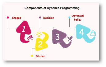
Components of Dynamic programming
|
Fig 3 - Components of Dynamic programming
- Stages: The problem can be divided into several subproblems, which are called stages. A stage is a small portion of a given problem. For example, in the shortest path problem, they were defined by the structure of the graph.
- States: Each stage has several states associated with it. The states for the shortest path problem was the node reached.
- Decision: At each stage, there can be multiple choices out of which one of the best decisions should be taken. The decision taken at every stage should be optimal; this is called a stage decision.
- Optimal policy: It is a rule which determines the decision at each stage; a policy is called an optimal policy if it is globally optimal. This is known as Bellman principle of optimality.
- Given the current state, the optimal choices for each of the remaining states does not depend on the previous states or decisions. In the shortest path problem, it was not necessary to know how we got a node only that we did.
- There exist a recursive relationship that identify the optimal decisions for stage j, given that stage j+1, has already been solved.
- The final stage must be solved by itself.
Development of Dynamic Programming Algorithm
It can be broken into four steps:
- Characterize the structure of an optimal solution.
- Recursively defined the value of the optimal solution. Like Divide and Conquer, divide the problem into two or more optimal parts recursively. This helps to determine what the solution will look like.
- Compute the value of the optimal solution from the bottom up (starting with the smallest subproblems)
- Construct the optimal solution for the entire problem form the computed values of smaller subproblems.
Applications of dynamic programming
- 0/1 knapsack problem
- Mathematical optimization problem
- All pair Shortest path problem
- Reliability design problem
- Longest common subsequence (LCS)
- Flight control and robotics control
- Time-sharing: It schedules the job to maximize CPU usage
Key takeaway
- Dynamic Programming is the most powerful design technique for solving optimization problems.
- Divide & Conquer algorithm partition the problem into disjoint subproblems solve the subproblems recursively and then combine their solution to solve the original problems.
- Dynamic Programming is used when the subproblems are not independent, e.g. when they share the same subproblems. In this case, divide and conquer may do more work than necessary, because it solves the same sub problem multiple times.
- Dynamic Programming solves each subproblems just once and stores the result in a table so that it can be repeatedly retrieved if needed again.
Branch and bound is an algorithm design paradigm which is generally used for solving combinatorial optimization problems. These problems are typically exponential in terms of time complexity and may require exploring all possible permutations in worst case. The Branch and Bound Algorithm technique solves these problems relatively quickly.
Let us consider the 0/1 Knapsack problem to understand Branch and Bound.
There are many algorithms by which the knapsack problem can be solved:
Greedy Algorithm for Fractional Knapsack
DP solution for 0/1 Knapsack
Backtracking Solution for 0/1 Knapsack.
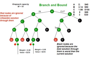
Let’s see the Branch and Bound Approach to solve the 0/1 Knapsack problem: The Backtracking Solution can be optimized if we know a bound on best possible solution subtree rooted with every node. If the best in subtree is worse than current best, we can simply ignore this node and its subtrees. So we compute bound (best solution) for every node and compare the bound with current best solution before exploring the node.
Example bounds used in below diagram are, A down can give $315, B down can $275, C down can $225, D down can $125 and E down can $30.
|
Key takeaway
- Branch and bound is an algorithm design paradigm which is generally used for solving combinatorial optimization problems. These problems are typically exponential in terms of time complexity and may require exploring all possible permutations in worst case. The Branch and Bound Algorithm technique solves these problems relatively quickly.
In Greedy Algorithm a set of resources are recursively divided based on the maximum, immediate availability of that resource at any given stage of execution.
To solve a problem based on the greedy approach, there are two stages
- Scanning the list of items
- Optimization
These stages are covered parallelly in this Greedy algorithm tutorial, on course of division of the array.
To understand the greedy approach, you will need to have a working knowledge of recursion and context switching. This helps you to understand how to trace the code. You can define the greedy paradigm in terms of your own necessary and sufficient statements.
Two conditions define the greedy paradigm.
- Each stepwise solution must structure a problem towards its best-accepted solution.
- It is sufficient if the structuring of the problem can halt in a finite number of greedy steps.
With the theorizing continued, let us describe the history associated with the Greedy search approach.
Here is an important landmark of greedy algorithms:
- Greedy algorithms were conceptualized for many graph walk algorithms in the 1950s.
- Esdger Djikstra conceptualized the algorithm to generate minimal spanning trees. He aimed to shorten the span of routes within the Dutch capital, Amsterdam.
- In the same decade, Prim and Kruskal achieved optimization strategies that were based on minimizing path costs along weighed routes.
- In the '70s, American researchers, Cormen, Rivest, and Stein proposed a recursive substructuring of greedy solutions in their classical introduction to algorithms book.
- The Greedy search paradigm was registered as a different type of optimization strategy in the NIST records in 2005.
- Till date, protocols that run the web, such as the open-shortest-path-first (OSPF) and many other network packet switching protocols use the greedy strategy to minimize time spent on a network.
Greedy Strategies and Decisions
Logic in its easiest form was boiled down to "greedy" or "not greedy". These statements were defined by the approach taken to advance in each algorithm stage.
For example, Djikstra's algorithm utilized a stepwise greedy strategy identifying hosts on the Internet by calculating a cost function. The value returned by the cost function determined whether the next path is "greedy" or "non-greedy".
In short, an algorithm ceases to be greedy if at any stage it takes a step that is not locally greedy. The Greedy problems halt with no further scope of greed.
Characteristics of the Greedy Approach
The important characteristics of a Greedy method algorithm are:
- There is an ordered list of resources, with costs or value attributions. These quantify constraints on a system.
- You will take the maximum quantity of resources in the time a constraint applies.
- For example, in an activity scheduling problem, the resource costs are in hours, and the activities need to be performed in serial order.
|
Fig 4 – Greedy method approach
Here are the reasons for using the greedy approach:
- The greedy approach has a few tradeoffs, which may make it suitable for optimization.
- One prominent reason is to achieve the most feasible solution immediately. In the activity selection problem (Explained below), if more activities can be done before finishing the current activity, these activities can be performed within the same time.
- Another reason is to divide a problem recursively based on a condition, with no need to combine all the solutions.
- In the activity selection problem, the "recursive division" step is achieved by scanning a list of items only once and considering certain activities.
How to Solve the activity selection problem
In the activity scheduling example, there is a "start" and "finish" time for every activity. Each Activity is indexed by a number for reference. There are two activity categories.
- considered activity: is the Activity, which is the reference from which the ability to do more than one remaining Activity is analyzed.
- remaining activities: activities at one or more indexes ahead of the considered activity.
The total duration gives the cost of performing the activity. That is (finish - start) gives us the durational as the cost of an activity.
You will learn that the greedy extent is the number of remaining activities you can perform in the time of a considered activity.
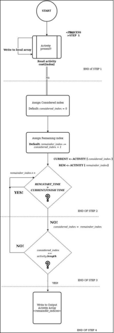
Architecture of the Greedy approach
STEP 1)
Scan the list of activity costs, starting with index 0 as the considered Index.
STEP 2)
When more activities can be finished by the time, the considered activity finishes, start searching for one or more remaining activities.
STEP 3)
If there are no more remaining activities, the current remaining activity becomes the next considered activity. Repeat step 1 and step 2, with the new considered activity. If there are no remaining activities left, go to step 4.
STEP 4 )
Return the union of considered indices. These are the activity indices that will be used to maximize throughput.
|
Fig 5 - Architecture of the Greedy Approach
#include<iostream>
#include<stdio.h>
#include<stdlib.h>
#define MAX_ACTIVITIES 12
|
Explanation of code:
- Included header files/classes
- A max number of activities provided by the user.
using namespace std;
class TIME
{
public:
int hours;
public: TIME()
{
hours = 0;
}
};
|
Explanation of code:
- The namespace for streaming operations.
- A class definition for TIME
- An hour timestamp.
- A TIME default constructor
- The hours variable.
class Activity
{
public:
int index;
TIME start;
TIME finish;
public: Activity()
{
start = finish = TIME();
}
};
|
Explanation of code:
- A class definition from activity
- Timestamps defining a duration
- All timestamps are initialized to 0 in the default constructor
class Scheduler
{
public:
int considered_index,init_index;
Activity *current_activities = new Activity[MAX_ACTIVITIES];
Activity *scheduled;
|
Explanation of code:
- Part 1 of the scheduler class definition.
- Considered Index is the starting point for scanning the array.
- The initialization index is used to assign random timestamps.
- An array of activity objects is dynamically allocated using the new operator.
- The scheduled pointer defines the current base location for greed.
Scheduler()
{
considered_index = 0;
scheduled = NULL;
...
...
|
Explanation of code:
- The scheduler constructor - part 2 of the scheduler class definition.
- The considered index defines the current start of the current scan.
- The current greedy extent is undefined at the start.
for(init_index = 0; init_index < MAX_ACTIVITIES; init_index++)
{
current_activities[init_index].start.hours =
rand() % 12;
current_activities[init_index].finish.hours =
current_activities[init_index].start.hours +
(rand() % 2);
printf("\nSTART:%d END %d\n",
current_activities[init_index].start.hours
,current_activities[init_index].finish.hours);
}
…
…
|
Explanation of code:
- A for loop to initialize start hours and end hours of each of the activities currently scheduled.
- Start time initialization.
- End time initialization always after or exactly at the start hour.
- A debug statement to print out allocated durations.
public:
Activity * activity_select(int);
};
|
Explanation of code:
- Part 4 - the last part of the scheduler class definition.
- Activity select function takes a starting point index as the base and divides the greedy quest into greedy subproblems.
Activity * Scheduler :: activity_select(int considered_index)
{
this->considered_index = considered_index;
int greedy_extent = this->considered_index + 1;
…
…
|
- Using the scope resolution operator (::), the function definition is provided.
- The considered Index is the Index called by value. The greedy_extent is the initialized just an index after the considered Index.
Activity * Scheduler :: activity_select(int considered_index)
{
while( (greedy_extent < MAX_ACTIVITIES ) &&
((this->current_activities[greedy_extent]).start.hours <
(this->current_activities[considered_index]).finish.hours ))
{
printf("\nSchedule start:%d \nfinish%d\n activity:%d\n",
(this->current_activities[greedy_extent]).start.hours,
(this->current_activities[greedy_extent]).finish.hours,
greedy_extent + 1);
greedy_extent++;
}
…
...
|
Explanation of code:
- The core logic- The greedy extent is limited to the number of activities.
- The start hours of the current Activity are checked as schedulable before the considered Activity (given by considered index) would finish.
- As long as this possible, an optional debug statement is printed.
- Advance to next index on the activity array
...
if ( greedy_extent <= MAX_ACTIVITIES )
{
return activity_select(greedy_extent);
}
else
{
return NULL;
}
}
|
Explanation of code:
- The conditional checks if all the activities have been covered.
- If not, you can restart your greedy with the considered Index as the current point. This is a recursive step that greedily divides the problem statement.
- If yes, it returns to the caller with no scope for extending greed.
int main()
{
Scheduler *activity_sched = new Scheduler();
activity_sched->scheduled = activity_sched->activity_select(
activity_sched->considered_index);
return 0;
}
|
Explanation of code:
- The main function used to invoke the scheduler.
- A new Scheduler is instantiated.
- The activity select function, which returns a pointer of type activity comes back to the caller after the greedy quest is over.
Output:
START:7 END 7
START:9 END 10
START:5 END 6
START:10 END 10
START:9 END 10
Schedule start:5
finish6
activity:3
Schedule start:9
finish10
activity:5
Disadvantages of Greedy Algorithms
It is not suitable for Greedy problems where a solution is required for every subproblem like sorting.
In such Greedy algorithm practice problems, the Greedy method can be wrong; in the worst case even lead to a non-optimal solution.
Therefore the disadvantage of greedy algorithms is using not knowing what lies ahead of the current greedy state.
Below is a depiction of the disadvantage of the Greedy method:
|
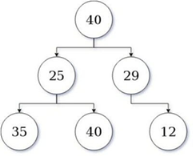
Fig 5 - Depiction of the disadvantage of the Greedy method
In the greedy scan shown here as a tree (higher value higher greed), an algorithm state at value: 40, is likely to take 29 as the next value. Further, its quest ends at 12. This amounts to a value of 41.
However, if the algorithm took a sub-optimal path or adopted a conquering strategy. then 25 would be followed by 40, and the overall cost improvement would be 65, which is valued 24 points higher as a suboptimal decision.
Most networking algorithms use the greedy approach. Here is a list of few Greedy algorithm examples:
- Prim's Minimal Spanning Tree Algorithm
- Travelling Salesman Problem
- Graph - Map Coloring
- Kruskal's Minimal Spanning Tree Algorithm
- Dijkstra's Minimal Spanning Tree Algorithm
- Graph - Vertex Cover
- Knapsack Problem
- Job Scheduling Problem
Summary:
To summarize, the article defined the greedy paradigm, showed how greedy optimization and recursion, can help you obtain the best solution up to a point. The Greedy algorithm is widely taken into application for problem solving in many languages as Greedy algorithm Python, C, C#, PHP, Java, etc. The activity selection of Greedy algorithm example was described as a strategic problem that could achieve maximum throughput using the greedy approach. In the end, the demerits of the usage of the greedy approach were explained.
Key takeaway
In Greedy Algorithm a set of resources are recursively divided based on the maximum, immediate availability of that resource at any given stage of execution.
To solve a problem based on the greedy approach, there are two stages
- Scanning the list of items
- Optimization
These stages are covered parallelly in this Greedy algorithm tutorial, on course of division of the array.
To understand the greedy approach, you will need to have a working knowledge of recursion and context switching. This helps you to understand how to trace the code. You can define the greedy paradigm in terms of your own necessary and sufficient statements.
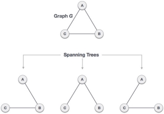
A spanning tree is a subset of Graph G, which has all the vertices covered with minimum possible number of edges. Hence, a spanning tree does not have cycles and it cannot be disconnected..
By this definition, we can draw a conclusion that every connected and undirected Graph G has at least one spanning tree. A disconnected graph does not have any spanning tree, as it cannot be spanned to all its vertices.
|
Fig 6 – Spanning Tree
We found three spanning trees off one complete graph. A complete undirected graph can have maximum nn-2 number of spanning trees, where n is the number of nodes. In the above addressed example, n is 3, hence 33−2 = 3 spanning trees are possible.
General Properties of Spanning Tree
We now understand that one graph can have more than one spanning tree. Following are a few properties of the spanning tree connected to graph G −
- A connected graph G can have more than one spanning tree.
- All possible spanning trees of graph G, have the same number of edges and vertices.
- The spanning tree does not have any cycle (loops).
- Removing one edge from the spanning tree will make the graph disconnected, i.e. the spanning tree is minimally connected.
- Adding one edge to the spanning tree will create a circuit or loop, i.e. the spanning tree is maximally acyclic.
Mathematical Properties of Spanning Tree
- Spanning tree has n-1 edges, where n is the number of nodes (vertices).
- From a complete graph, by removing maximum e - n + 1 edges, we can construct a spanning tree.
- A complete graph can have maximum nn-2 number of spanning trees.
Thus, we can conclude that spanning trees are a subset of connected Graph G and disconnected graphs do not have spanning tree.
Spanning tree is basically used to find a minimum path to connect all nodes in a graph. Common application of spanning trees are −
- Civil Network Planning
- Computer Network Routing Protocol
- Cluster Analysis
Let us understand this through a small example. Consider, city network as a huge graph and now plans to deploy telephone lines in such a way that in minimum lines we can connect to all city nodes. This is where the spanning tree comes into picture.
In a weighted graph, a minimum spanning tree is a spanning tree that has minimum weight than all other spanning trees of the same graph. In real-world situations, this weight can be measured as distance, congestion, traffic load or any arbitrary value denoted to the edges.
Minimum Spanning-Tree Algorithm
We shall learn about two most important spanning tree algorithms here −
- Kruskal's Algorithm
- Prim's Algorithm
Both are greedy algorithms.
Key takeaway
A spanning tree is a subset of Graph G, which has all the vertices covered with minimum possible number of edges. Hence, a spanning tree does not have cycles and it cannot be disconnected..
By this definition, we can draw a conclusion that every connected and undirected Graph G has at least one spanning tree. A disconnected graph does not have any spanning tree, as it cannot be spanned to all its vertices.
Knapsack is basically means bag. A bag of given capacity.
We want to pack n items in your luggage.
- The ith item is worth vi dollars and weight wi pounds.
- Take as valuable a load as possible, but cannot exceed W pounds.
- vi wi W are integers.
- W ≤ capacity
- Value ← Max
Input:
- Knapsack of capacity
- List (Array) of weight and their corresponding value.
Output: To maximize profit and minimize weight in capacity.
The knapsack problem where we have to pack the knapsack with maximum value in such a manner that the total weight of the items should not be greater than the capacity of the knapsack.
Knapsack problem can be further divided into two parts:
1. Fractional Knapsack: Fractional knapsack problem can be solved by Greedy Strategy where as 0 /1 problem is not.
It cannot be solved by Dynamic Programming Approach.
In this item cannot be broken which means thief should take the item as a whole or should leave it. That's why it is called 0/1 knapsack Problem.
- Each item is taken or not taken.
- Cannot take a fractional amount of an item taken or take an item more than once.
- It cannot be solved by the Greedy Approach because it is enable to fill the knapsack to capacity.
- Greedy Approach doesn't ensure an Optimal Solution.
Example of 0/1 Knapsack Problem:
Example: The maximum weight the knapsack can hold is W is 11. There are five items to choose from. Their weights and values are presented in the following table:
|
The [i, j] entry here will be V [i, j], the best value obtainable using the first "i" rows of items if the maximum capacity were j. We begin by initialization and first row.
V [i, j] = max {V [i - 1, j], vi + V [i - 1, j -wi]
The value of V [3, 7] was computed as follows: V [3, 7] = max {V [3 - 1, 7], v3 + V [3 - 1, 7 - w3] = max {V [2, 7], 18 + V [2, 7 - 5]} = max {7, 18 + 6} = 24
Finally, the output is:
|
The maximum value of items in the knapsack is 40, the bottom-right entry). The dynamic programming approach can now be coded as the following algorithm:
KNAPSACK (n, W)
1. for w = 0, W
2. do V [0,w] ← 0
3. for i=0, n
4. do V [i, 0] ← 0
5. for w = 0, W
6. do if (wi≤ w & vi + V [i-1, w - wi]> V [i -1,W])
7. then V [i, W] ← vi + V [i - 1, w - wi]
8. else V [i, W] ← V [i - 1, w]
Key takeaway
Knapsack is basically means bag. A bag of given capacity.
We want to pack n items in your luggage.
- The ith item is worth vi dollars and weight wi pounds.
- Take as valuable a load as possible, but cannot exceed W pounds.
- vi wi W are integers.
3. W ≤ capacity
4. Value ← Max
Input:
- Knapsack of capacity
- List (Array) of weight and their corresponding value.
Output: To maximize profit and minimize weight in capacity.
In job sequencing problem, the objective is to find a sequence of jobs, which is completed within their deadlines and gives maximum profit.
Let us consider, a set of n given jobs which are associated with deadlines and profit is earned, if a job is completed by its deadline. These jobs need to be ordered in such a way that there is maximum profit.
It may happen that all of the given jobs may not be completed within their deadlines.
Assume, deadline of ith job Ji is di and the profit received from this job is pi. Hence, the optimal solution of this algorithm is a feasible solution with maximum profit.
Thus, D(i)>0
for 1⩽i⩽n
.Initially, these jobs are ordered according to profit, i.e. p1⩾p2⩾p3⩾...⩾pn
.Algorithm: Job-Sequencing-With-Deadline (D, J, n, k)
D(0) := J(0) := 0
k := 1
J(1) := 1 // means first job is selected
for i = 2 … n do
r := k
while D(J(r)) > D(i) and D(J(r)) ≠ r do
r := r – 1
if D(J(r)) ≤ D(i) and D(i) > r then
for l = k … r + 1 by -1 do
J(l + 1) := J(l)
J(r + 1) := i
k := k + 1
In this algorithm, we are using two loops, one is within another. Hence, the complexity of this algorithm is O(n2)
Example
Let us consider a set of given jobs as shown in the following table. We have to find a sequence of jobs, which will be completed within their deadlines and will give maximum profit. Each job is associated with a deadline and profit.
Job | J1 | J2 | J3 | J4 | J5 |
Deadline | 2 | 1 | 3 | 2 | 1 |
Profit | 60 | 100 | 20 | 40 | 20 |
To solve this problem, the given jobs are sorted according to their profit in a descending order. Hence, after sorting, the jobs are ordered as shown in the following table.
Job | J2 | J1 | J4 | J3 | J5 |
Deadline | 1 | 2 | 2 | 3 | 1 |
Profit | 100 | 60 | 40 | 20 | 20 |
From this set of jobs, first we select J2, as it can be completed within its deadline and contributes maximum profit.
- Next, J1 is selected as it gives more profit compared to J4.
- In the next clock, J4 cannot be selected as its deadline is over, hence J3 is selected as it executes within its deadline.
- The job J5 is discarded as it cannot be executed within its deadline.
Thus, the solution is the sequence of jobs (J2, J1, J3), which are being executed within their deadline and gives maximum profit.
Total profit of this sequence is 100 + 60 + 20 = 180.
Key takeaway
Algorithm: Job-Sequencing-With-Deadline (D, J, n, k)
D(0) := J(0) := 0
k := 1
J(1) := 1 // means first job is selected
for i = 2 … n do
r := k
while D(J(r)) > D(i) and D(J(r)) ≠ r do
r := r – 1
if D(J(r)) ≤ D(i) and D(i) > r then
for l = k … r + 1 by -1 do
J(l + 1) := J(l)
J(r + 1) := i
k := k + 1
- i) Data can be encoded efficiently using Huffman Codes.
- (ii) It is a widely used and beneficial technique for compressing data.
- (iii) Huffman's greedy algorithm uses a table of the frequencies of occurrences of each character to build up an optimal way of representing each character as a binary string.
Suppose we have 105 characters in a data file. Normal Storage: 8 bits per character (ASCII) - 8 x 105 bits in a file. But we want to compress the file and save it compactly. Suppose only six characters appear in the file:
|
How can we represent the data in a Compact way?
(i) Fixed length Code: Each letter represented by an equal number of bits. With a fixed length code, at least 3 bits per character:
For example:
a 000
b 001
c 010
d 011
e 100
f 101
For a file with 105 characters, we need 3 x 105 bits.
(ii) A variable-length code: It can do considerably better than a fixed-length code, by giving many characters short code words and infrequent character long codewords.
For example:
a 0
b 101
c 100
d 111
e 1101
f 1100
Number of bits = (45 x 1 + 13 x 3 + 12 x 3 + 16 x 3 + 9 x 4 + 5 x 4) x 1000
= 2.24 x 105bits
Thus, 224,000 bits to represent the file, a saving of approximately 25%.This is an optimal character code for this file.
The prefixes of an encoding of one character must not be equal to complete encoding of another character, e.g., 1100 and 11001 are not valid codes because 1100 is a prefix of some other code word is called prefix codes.
Prefix codes are desirable because they clarify encoding and decoding. Encoding is always simple for any binary character code; we concatenate the code words describing each character of the file. Decoding is also quite comfortable with a prefix code. Since no codeword is a prefix of any other, the codeword that starts with an encoded data is unambiguous.
Greedy Algorithm for constructing a Huffman Code:
Huffman invented a greedy algorithm that creates an optimal prefix code called a Huffman Code.
|
Fig 7 – Greedy Algorithm for constructing a Huffman Code
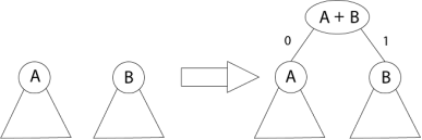
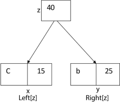
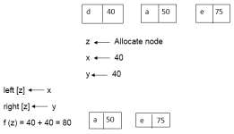
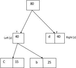
The algorithm builds the tree T analogous to the optimal code in a bottom-up manner. It starts with a set of |C| leaves (C is the number of characters) and performs |C| - 1 'merging' operations to create the final tree. In the Huffman algorithm 'n' denotes the quantity of a set of characters, z indicates the parent node, and x & y are the left & right child of z respectively.
Huffman (C)
1. n=|C|
2. Q ← C
3. for i=1 to n-1
4. do
5. z= allocate-Node ()
6. x= left[z]=Extract-Min(Q)
7. y= right[z] =Extract-Min(Q)
8. f [z]=f[x]+f[y]
9. Insert (Q, z)
10. return Extract-Min (Q)
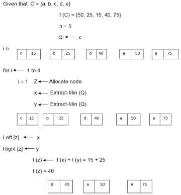
Example: Find an optimal Huffman Code for the following set of frequencies:
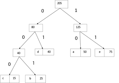
- a: 50 b: 25 c: 15 d: 40 e: 75
Solution:
|
i.e.
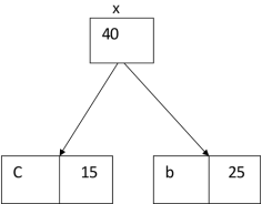
Again for i=2
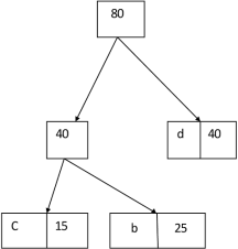
Similarly, we apply the same process we get
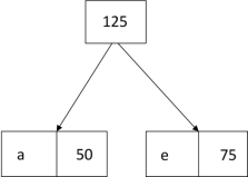
Thus, the final output is:
|
Key takeaway
- (i) Data can be encoded efficiently using Huffman Codes.
- (ii) It is a widely used and beneficial technique for compressing data.
- (iii) Huffman's greedy algorithm uses a table of the frequencies of occurrences of each character to build up an optimal way of representing each character as a binary string.
In a shortest- paths problem, we are given a weighted, directed graphs G = (V, E), with weight function w: E → R mapping edges to real-valued weights. The weight of path p = (v0,v1,..... vk) is the total of the weights of its constituent edges:

We define the shortest - path weight from u to v by δ(u,v) = min (w (p): u→v), if there is a path from u to v, and δ(u,v)= ∞, otherwise.
The shortest path from vertex s to vertex t is then defined as any path p with weight w (p) = δ(s,t).
The breadth-first- search algorithm is the shortest path algorithm that works on unweighted graphs, that is, graphs in which each edge can be considered to have unit weight.
In a Single Source Shortest Paths Problem, we are given a Graph G = (V, E), we want to find the shortest path from a given source vertex s ∈ V to every vertex v ∈ V.
There are some variants of the shortest path problem.
- Single- destination shortest - paths problem: Find the shortest path to a given destination vertex t from every vertex v. By shift the direction of each edge in the graph, we can shorten this problem to a single - source problem.
- Single - pair shortest - path problem: Find the shortest path from u to v for given vertices u and v. If we determine the single - source problem with source vertex u, we clarify this problem also. Furthermore, no algorithms for this problem are known that run asymptotically faster than the best single - source algorithms in the worst case.
- All - pairs shortest - paths problem: Find the shortest path from u to v for every pair of vertices u and v. Running a single - source algorithm once from each vertex can clarify this problem; but it can generally be solved faster, and its structure is of interest in the own right.
If some path from s to v contains a negative cost cycle then, there does not exist the shortest path. Otherwise, there exists a shortest s - v that is simple.
|
Fig 8 - Shortest Path: Existence
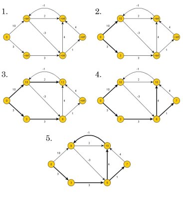
The single source shortest path algorithm (for arbitrary weight positive or negative) is also known Bellman-Ford algorithm is used to find minimum distance from source vertex to any other vertex. The main difference between this algorithm with Dijkstra’s algorithm is, in Dijkstra’s algorithm we cannot handle the negative weight, but here we can handle it easily.
|
Fig 9 - The single source shortest path algorithm
Bellman-Ford algorithm finds the distance in bottom up manner. At first it finds those distances which have only one edge in the path. After that increase the path length to find all possible solutions.
Input − The cost matrix of the graph:
0 6 ∞ 7 ∞
∞ 0 5 8 -4
∞ -2 0 ∞ ∞
∞ ∞ -3 0 9
2 ∞ 7 ∞ 0
Output − Source Vertex: 2
Vert: 0 1 2 3 4
Dist: -4 -2 0 3 -6
Pred: 4 2 -1 0 1
The graph has no negative edge cycle
bellmanFord(dist, pred, source) Input − Distance list, predecessor list and the source vertex. Output − True, when a negative cycle is found. Begin iCount := 1 maxEdge := n * (n - 1) / 2 //n is number of vertices for all vertices v of the graph, do dist[v] := ∞ pred[v] := ϕ done dist[source] := 0 eCount := number of edges present in the graph create edge list named edgeList while iCount < n, do for i := 0 to eCount, do if dist[edgeList[i].v] > dist[edgeList[i].u] + (cost[u,v] for edge i) dist[edgeList[i].v] > dist[edgeList[i].u] + (cost[u,v] for edge i) pred[edgeList[i].v] := edgeList[i].u done done iCount := iCount + 1 for all vertices i in the graph, do if dist[edgeList[i].v] > dist[edgeList[i].u] + (cost[u,v] for edge i), then return true done return false End #include<iostream> #include<iomanip> #define V 5 #define INF 999 using namespace std; //Cost matrix of the graph (directed) vertex 5 int costMat[V][V] = { {0, 6, INF, 7, INF}, {INF, 0, 5, 8, -4}, {INF, -2, 0, INF, INF}, {INF, INF, -3, 0, 9}, {2, INF, 7, INF, 0} }; typedef struct{ int u, v, cost; }edge; int isDiagraph(){ //check the graph is directed graph or not int i, j; for(i = 0; i<V; i++){ for(j = 0; j<V; j++){ if(costMat[i][j] != costMat[j][i]){ return 1;//graph is directed } } } return 0;//graph is undirected } int makeEdgeList(edge *eList){ //create edgelist from the edges of graph int count = -1; if(isDiagraph()){ for(int i = 0; i<V; i++){ for(int j = 0; j<V; j++){ if(costMat[i][j] != 0 && costMat[i][j] != INF){ count++;//edge find when graph is directed eList[count].u = i; eList[count].v = j; eList[count].cost = costMat[i][j]; } } } }else{ for(int i = 0; i<V; i++){ for(int j = 0; j<i; j++){ if(costMat[i][j] != INF){ count++;//edge find when graph is undirected eList[count].u = i; eList[count].v = j; eList[count].cost = costMat[i][j]; } } } } return count+1; } int bellmanFord(int *dist, int *pred,int src){ int icount = 1, ecount, max = V*(V-1)/2; edge edgeList[max]; for(int i = 0; i<V; i++){ dist[i] = INF;//initialize with infinity pred[i] = -1;//no predecessor found. } dist[src] = 0;//for starting vertex, distance is 0 ecount = makeEdgeList(edgeList); //edgeList formation while(icount < V){ //number of iteration is (Vertex - 1) for(int i = 0; i<ecount; i++){ if(dist[edgeList[i].v] > dist[edgeList[i].u] + costMat[edgeList[i].u][edgeList[i].v]){ //relax edge and set predecessor dist[edgeList[i].v] = dist[edgeList[i].u] + costMat[edgeList[i].u][edgeList[i].v]; pred[edgeList[i].v] = edgeList[i].u; } } icount++; } //test for negative cycle for(int i = 0; i<ecount; i++){ if(dist[edgeList[i].v] > dist[edgeList[i].u] + costMat[edgeList[i].u][edgeList[i].v]){ return 1;//indicates the graph has negative cycle } } return 0;//no negative cycle } void display(int *dist, int *pred){ cout << "Vert: "; for(int i = 0; i<V; i++) cout <<setw(3) << i << " "; cout << endl; cout << "Dist: "; for(int i = 0; i<V; i++) cout << setw(3) << dist[i] << " "; cout << endl; cout << "Pred: "; for(int i = 0; i<V; i++) cout << setw(3) << pred[i] << " "; cout << endl; } int main(){ int dist[V], pred[V], source, report; source = 2; report = bellmanFord(dist, pred, source); cout << "Source Vertex: " << source<<endl; display(dist, pred); if(report) cout << "The graph has a negative edge cycle" << endl; else cout << "The graph has no negative edge cycle" << endl; }
|
Source Vertex: 2
Vert: 0 1 2 3 4
Dist: -4 -2 0 3 -6
Pred: 4 2 -1 0 1
The graph has no negative edge cycle
Key takeaway
In a shortest- paths problem, we are given a weighted, directed graphs G = (V, E), with weight function w: E → R mapping edges to real-valued weights. The weight of path p = (v0,v1,..... vk) is the total of the weights of its constituent edges:

We define the shortest - path weight from u to v by δ(u,v) = min (w (p): u→v), if there is a path from u to v, and δ(u,v)= ∞, otherwise.
The shortest path from vertex s to vertex t is then defined as any path p with weight w (p) = δ(s,t).
The breadth-first- search algorithm is the shortest path algorithm that works on unweighted graphs, that is, graphs in which each edge can be considered to have unit weight.
In a Single Source Shortest Paths Problem, we are given a Graph G = (V, E), we want to find the shortest path from a given source vertex s ∈ V to every vertex v ∈ V.
Dynamic programming approach is similar to divide and conquer in breaking down the problem into smaller and yet smaller possible sub-problems. But unlike, divide and conquer, these sub-problems are not solved independently. Rather, results of these smaller sub-problems are remembered and used for similar or overlapping sub-problems.
Dynamic programming is used where we have problems, which can be divided into similar sub-problems, so that their results can be re-used. Mostly, these algorithms are used for optimization. Before solving the in-hand sub-problem, dynamic algorithm will try to examine the results of the previously solved sub-problems. The solutions of sub-problems are combined in order to achieve the best solution.
So we can say that −
- The problem should be able to be divided into smaller overlapping sub-problem.
- An optimum solution can be achieved by using an optimum solution of smaller sub-problems.
- Dynamic algorithms use Memoization.
In contrast to greedy algorithms, where local optimization is addressed, dynamic algorithms are motivated for an overall optimization of the problem.
In contrast to divide and conquer algorithms, where solutions are combined to achieve an overall solution, dynamic algorithms use the output of a smaller sub-problem and then try to optimize a bigger sub-problem. Dynamic algorithms use Memoization to remember the output of already solved sub-problems.
The following computer problems can be solved using dynamic programming approach −
- Fibonacci number series
- Knapsack problem
- Tower of Hanoi
- All pair shortest path by Floyd-Warshall
- Shortest path by Dijkstra
- Project scheduling
Dynamic programming can be used in both top-down and bottom-up manner. And of course, most of the times, referring to the previous solution output is cheaper than recomputing in terms of CPU cycles.
Key takeaway
Dynamic programming approach is similar to divide and conquer in breaking down the problem into smaller and yet smaller possible sub-problems. But unlike, divide and conquer, these sub-problems are not solved independently. Rather, results of these smaller sub-problems are remembered and used for similar or overlapping sub-problems.
Dynamic programming is used where we have problems, which can be divided into similar sub-problems, so that their results can be re-used. Mostly, these algorithms are used for optimization. Before solving the in-hand sub-problem, dynamic algorithm will try to examine the results of the previously solved sub-problems. The solutions of sub-problems are combined in order to achieve the best solution.
Divide & Conquer Method | Dynamic Programming |
1.It deals (involves) three steps at each level of recursion: | 1.It involves the sequence of four steps:
|
2. It is Recursive. | 2. It is non Recursive. |
3. It does more work on subproblems and hence has more time consumption. | 3. It solves subproblems only once and then stores in the table. |
4. It is a top-down approach. | 4. It is a Bottom-up approach. |
5. In this subproblems are independent of each other. | 5. In this subproblems are interdependent. |
6. For example: Merge Sort & Binary Search etc. | 6. For example: Matrix Multiplication. |
Key takeaway
Divide & Conquer Method | Dynamic Programming |
1.It deals (involves) three steps at each level of recursion: | 1.It involves the sequence of four steps:
|
Fibonacci sequence is the sequence of numbers in which every next item is the total of the previous two items. And each number of the Fibonacci sequence is called Fibonacci number.
Example: 0 ,1,1,2,3,5,8,13,21,....................... is a Fibonacci sequence.
The Fibonacci numbers F_nare defined as follows:
F0 = 0
Fn=1
Fn=F(n-1)+ F(n-2)
FIB (n)
1. If (n < 2)
2. then return n
3. else return FIB (n - 1) + FIB (n - 2)
Figure 10 : shows four levels of recursion for the call fib (8):
|
Figure: Recursive calls during computation of Fibonacci number
A single recursive call to fib (n) results in one recursive call to fib (n - 1), two recursive calls to fib (n - 2), three recursive calls to fib (n - 3), five recursive calls to fib (n - 4) and, in general, Fk-1 recursive calls to fib (n - k) We can avoid this unneeded repetition by writing down the conclusion of recursive calls and looking them up again if we need them later. This process is called memorization.
Here is the algorithm with memorization
MEMOFIB (n)
1 if (n < 2)
2 then return n
3 if (F[n] is undefined)
4 then F[n] ← MEMOFIB (n - 1) + MEMOFIB (n - 2)
5 return F[n]
If we trace through the recursive calls to MEMOFIB, we find that array F [] gets filled from bottom up. I.e., first F [2], then F [3], and so on, up to F[n]. We can replace recursion with a simple for-loop that just fills up the array F [] in that order
ITERFIB (n)
1 F [0] ← 0
2 F [1] ← 1
3 for i ← 2 to n
4 do
5 F[i] ← F [i - 1] + F [i - 2]
6 return F[n]
This algorithm clearly takes only O (n) time to compute Fn. By contrast, the original recursive algorithm takes O (∅n;),∅ =  = 1.618. ITERFIB conclude an exponential speedup over the original recursive algorithm.
Example: We are given the sequence {4, 10, 3, 12, 20, and 7}. The matrices have size 4 x 10, 10 x 3, 3 x 12, 12 x 20, 20 x 7. We need to compute M [i,j], 0 ≤ i, j≤ 5. We know M [i, i] = 0 for all i.
|
Let us proceed with working away from the diagonal. We compute the optimal solution for the product of 2 matrices.
|
Here P0 to P5 are Position and M1 to M5 are matrix of size (pi to pi-1)
On the basis of sequence, we make a formula

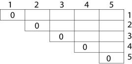
In Dynamic Programming, initialization of every method done by '0'.So we initialize it by '0'.It will sort out diagonally.
We have to sort out all the combination but the minimum output combination is taken into consideration.
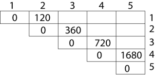
Calculation of Product of 2 matrices:
1. m (1,2) = m1 x m2
= 4 x 10 x 10 x 3
= 4 x 10 x 3 = 120
2. m (2, 3) = m2 x m3
= 10 x 3 x 3 x 12
= 10 x 3 x 12 = 360
3. m (3, 4) = m3 x m4
= 3 x 12 x 12 x 20
= 3 x 12 x 20 = 720
4. m (4,5) = m4 x m5
= 12 x 20 x 20 x 7
= 12 x 20 x 7 = 1680
|
- We initialize the diagonal element with equal i,j value with '0'.
- After that second diagonal is sorted out and we get all the values corresponded to it
Now the third diagonal will be solved out in the same way.
Now product of 3 matrices:
M [1, 3] = M1 M2 M3
- There are two cases by which we can solve this multiplication: ( M1 x M2) + M3, M1+ (M2x M3)
- After solving both cases we choose the case in which minimum output is there.
|
M [1, 3] =264
As Comparing both output 264 is minimum in both cases so we insert 264 in table and ( M1 x M2) + M3 this combination is chosen for the output making.
M [2, 4] = M2 M3 M4
- There are two cases by which we can solve this multiplication: (M2x M3)+M4, M2+(M3 x M4)
- After solving both cases we choose the case in which minimum output is there.
|
M [2, 4] = 1320
As Comparing both output 1320 is minimum in both cases so we insert 1320 in table and M2+(M3 x M4) this combination is chosen for the output making.
M [3, 5] = M3 M4 M5
- There are two cases by which we can solve this multiplication: ( M3 x M4) + M5, M3+ ( M4xM5)
- After solving both cases we choose the case in which minimum output is there.
|
M [3, 5] = 1140
As Comparing both output 1140 is minimum in both cases so we insert 1140 in table and ( M3 x M4) + M5this combination is chosen for the output making.
|
Now Product of 4 matrices:
M [1, 4] = M1 M2 M3 M4
There are three cases by which we can solve this multiplication:
- ( M1 x M2 x M3) M4
- M1 x(M2 x M3 x M4)
- (M1 xM2) x ( M3 x M4)
After solving these cases we choose the case in which minimum output is there
|
M [1, 4] =1080
As comparing the output of different cases then '1080' is minimum output, so we insert 1080 in the table and (M1 xM2) x (M3 x M4) combination is taken out in output making,
M [2, 5] = M2 M3 M4 M5
There are three cases by which we can solve this multiplication:
- (M2 x M3 x M4)x M5
- M2 x( M3 x M4 x M5)
- (M2 x M3)x ( M4 x M5)
After solving these cases we choose the case in which minimum output is there
|
M [2, 5] = 1350
As comparing the output of different cases then '1350' is minimum output, so we insert 1350 in the table and M2 x( M3 x M4 xM5)combination is taken out in output making.
|
Now Product of 5 matrices:
M [1, 5] = M1 M2 M3 M4 M5
There are five cases by which we can solve this multiplication:
- (M1 x M2 xM3 x M4 )x M5
- M1 x( M2 xM3 x M4 xM5)
- (M1 x M2 xM3)x M4 xM5
- M1 x M2x(M3 x M4 xM5)
After solving these cases we choose the case in which minimum output is there
|
M [1, 5] = 1344
As comparing the output of different cases then '1344' is minimum output, so we insert 1344 in the table and M1 x M2 x(M3 x M4 x M5)combination is taken out in output making.
Final Output is:
|
Step 3: Computing Optimal Costs: let us assume that matrix Ai has dimension pi-1x pi for i=1, 2, 3....n. The input is a sequence (p0,p1,......pn) where length [p] = n+1. The procedure uses an auxiliary table m [1....n, 1.....n] for storing m [i, j] costs an auxiliary table s [1.....n, 1.....n] that record which index of k achieved the optimal costs in computing m [i, j].
The algorithm first computes m [i, j] ← 0 for i=1, 2, 3.....n, the minimum costs for the chain of length 1.
Algorithm of Matrix Chain Multiplication
MATRIX-CHAIN-ORDER (p)
1. n length[p]-1
2. for i ← 1 to n
3. do m [i, i] ← 0
4. for l ← 2 to n // l is the chain length
5. do for i ← 1 to n-l + 1
6. do j ← i+ l -1
7. m[i,j] ← ∞
8. for k ← i to j-1
9. do q ← m [i, k] + m [k + 1, j] + pi-1 pk pj
10. If q < m [i,j]
11. then m [i,j] ← q
12. s [i,j] ← k
13. return m and s.
We will use table s to construct an optimal solution.
Step 1: Constructing an Optimal Solution:
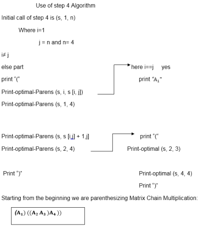
PRINT-OPTIMAL-PARENS (s, i, j)
1. if i=j
2. then print "A"
3. else print "("
4. PRINT-OPTIMAL-PARENS (s, i, s [i, j])
5. PRINT-OPTIMAL-PARENS (s, s [i, j] + 1, j)
6. print ")"
Analysis: There are three nested loops. Each loop executes a maximum n times.
- l, length, O (n) iterations.
- i, start, O (n) iterations.
- k, split point, O (n) iterations
Body of loop constant complexity
Total Complexity is: O (n3)
Algorithm with Explained Example
Question: P [7, 1, 5, 4, 2}
Solution: Here, P is the array of a dimension of matrices.
So here we will have 4 matrices:
A17x1 A21x5 A35x4 A44x2
i.e.
First Matrix A1 have dimension 7 x 1
Second Matrix A2 have dimension 1 x 5
Third Matrix A3 have dimension 5 x 4
Fourth Matrix A4 have dimension 4 x 2
Let say,
From P = {7, 1, 5, 4, 2} - (Given)
And P is the Position
p0 = 7, p1 =1, p2 = 5, p3 = 4, p4=2.
Length of array P = number of elements in P
∴length (p)= 5
From step 3
Follow the steps in Algorithm in Sequence
According to Step 1 of Algorithm Matrix-Chain-Order
Step 1:
n ← length [p]-1
Where n is the total number of elements
And length [p] = 5
∴ n = 5 - 1 = 4
n = 4
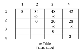
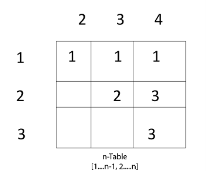
Now we construct two tables m and s.
Table m has dimension [1.....n, 1.......n]
Table s has dimension [1.....n-1, 2.......n]
|
Now, according to step 2 of Algorithm
- for i ← 1 to n
- this means: for i ← 1 to 4 (because n =4)
- for i=1
- m [i, i]=0
- m [1, 1]=0
- Similarly for i = 2, 3, 4
- m [2, 2] = m [3,3] = m [4,4] = 0
- i.e. fill all the diagonal entries "0" in the table m
- Now,
- l ← 2 to n
- l ← 2 to 4 (because n =4 )
Case 1:
1. When l - 2
for (i ← 1 to n - l + 1)
i ← 1 to 4 - 2 + 1
i ← 1 to 3
When i = 1
do j ← i + l - 1
j ← 1 + 2 - 1
j ← 2
i.e. j = 2
Now, m [i, j] ← ∞
i.e. m [1,2] ← ∞
Put ∞ in m [1, 2] table
for k ← i to j-1
k ← 1 to 2 - 1
k ← 1 to 1
k = 1
Now q ← m [i, k] + m [k + 1, j] + pi-1 pk pj
for l = 2
i = 1
j =2
k = 1
q ← m [1,1] + m [2,2] + p0x p1x p2
and m [1,1] = 0
for i ← 1 to 4
∴ q ← 0 + 0 + 7 x 1 x 5
q ← 35
We have m [i, j] = m [1, 2] = ∞
Comparing q with m [1, 2]
q < m [i, j]
i.e. 35 < m [1, 2]
35 < ∞
True
then, m [1, 2 ] ← 35 (∴ m [i,j] ← q)
s [1, 2] ← k
and the value of k = 1
s [1,2 ] ← 1
Insert "1" at dimension s [1, 2] in table s. And 35 at m [1, 2]
2. l remains 2
L = 2
i ← 1 to n - l + 1
i ← 1 to 4 - 2 + 1
i ← 1 to 3
for i = 1 done before
Now value of i becomes 2
i = 2
j ← i + l - 1
j ← 2 + 2 - 1
j ← 3
j = 3
m [i , j] ← ∞
i.e. m [2,3] ← ∞
Initially insert ∞ at m [2, 3]
Now, for k ← i to j - 1
k ← 2 to 3 - 1
k ← 2 to 2
i.e. k =2
Now, q ← m [i, k] + m [k + 1, j] + pi-1 pk pj
For l =2
i = 2
j = 3
k = 2
q ← m [2, 2] + m [3, 3] + p1x p2 x p3
q ← 0 + 0 + 1 x 5 x 4
q ← 20
Compare q with m [i ,j ]
If q < m [i,j]
i.e. 20 < m [2, 3]
20 < ∞
True
Then m [i,j ] ← q
m [2, 3 ] ← 20
and s [2, 3] ← k
and k = 2
s [2,3] ← 2
3. Now i become 3
i = 3
l = 2
j ← i + l - 1
j ← 3 + 2 - 1
j ← 4
j = 4
Now, m [i, j ] ← ∞
m [3,4 ] ← ∞
Insert ∞ at m [3, 4]
for k ← i to j - 1
k ← 3 to 4 - 1
k ← 3 to 3
i.e. k = 3
Now, q ← m [i, k] + m [k + 1, j] + pi-1 pk pj
i = 3
l = 2
j = 4
k = 3
q ← m [3, 3] + m [4,4] + p2 x p3 x p4
q ← 0 + 0 + 5 x 2 x 4
q 40
Compare q with m [i, j]
If q < m [i, j]
40 < m [3, 4]
40 < ∞
True
Then, m [i,j] ← q
m [3,4] ← 40
and s [3,4] ← k
s [3,4] ← 3
Case 2: l becomes 3
L = 3
for i = 1 to n - l + 1
i = 1 to 4 - 3 + 1
i = 1 to 2
When i = 1
j ← i + l - 1
j ← 1 + 3 - 1
j ← 3
j = 3
Now, m [i,j] ← ∞
m [1, 3] ← ∞
for k ← i to j - 1
k ← 1 to 3 - 1
k ← 1 to 2
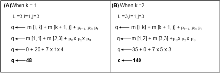
Now we compare the value for both k=1 and k = 2. The minimum of two will be placed in m [i,j] or s [i,j] respectively.
|
Now from above
Value of q become minimum for k=1
∴ m [i,j] ← q
m [1,3] ← 48
Also m [i,j] > q
i.e. 48 < ∞
∴ m [i , j] ← q
m [i, j] ← 48
and s [i,j] ← k
i.e. m [1,3] ← 48
s [1, 3] ← 1
Now i become 2
i = 2
l = 3
then j ← i + l -1
j ← 2 + 3 - 1
j ← 4
j = 4
so m [i,j] ← ∞
m [2,4] ← ∞
Insert initially ∞ at m [2, 4]
for k ← i to j-1
k ← 2 to 4 - 1
k ← 2 to 3
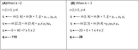
Here, also find the minimum value of m [i,j] for two values of k = 2 and k =3
|
- But 28 < ∞
- So m [i,j] ← q
- And q ← 28
- m [2, 4] ← 28
- and s [2, 4] ← 3
- e. It means in s table at s [2,4] insert 3 and at m [2,4] insert 28.
Case 3: l becomes 4
L = 4
For i ← 1 to n-l + 1
i ← 1 to 4 - 4 + 1
i ← 1
i = 1
do j ← i + l - 1
j ← 1 + 4 - 1
j ← 4
j = 4
Now m [i,j] ← ∞
m [1,4] ← ∞
for k ← i to j -1
k ← 1 to 4 - 1
k ← 1 to 3
When k = 1
q ← m [i, k] + m [k + 1, j] + pi-1 pk pj
q ← m [1,1] + m [2,4] + p0xp4x p1
q ← 0 + 28 + 7 x 2 x 1
q ← 42
Compare q and m [i, j]
m [i,j] was ∞
i.e. m [1,4]
if q < m [1,4]
42< ∞
True
Then m [i,j] ← q
m [1,4] ← 42
and s [1,4] 1 ? k =1
When k = 2
L = 4, i=1, j = 4
q ← m [i, k] + m [k + 1, j] + pi-1 pk pj
q ← m [1, 2] + m [3,4] + p0 xp2 xp4
q ← 35 + 40 + 7 x 5 x 2
q ← 145
Compare q and m [i,j]
Now m [i, j]
i.e. m [1,4] contains 42.
So if q < m [1, 4]
But 145 less than or not equal to m [1, 4]
So 145 less than or not equal to 42.
So no change occurs.
When k = 3
l = 4
i = 1
j = 4
q ← m [i, k] + m [k + 1, j] + pi-1 pk pj
q ← m [1, 3] + m [4,4] + p0 xp3 x p4
q ← 48 + 0 + 7 x 4 x 2
q ← 114
Again q less than or not equal to m [i, j]
i.e. 114 less than or not equal to m [1, 4]
114 less than or not equal to 42
So no change occurs. So the value of m [1, 4] remains 42. And value of s [1, 4] = 1
Now we will make use of only s table to get an optimal solution.
|
A subsequence of a given sequence is just the given sequence with some elements left out.
Given two sequences X and Y, we say that the sequence Z is a common sequence of X and Y if Z is a subsequence of both X and Y.
In the longest common subsequence problem, we are given two sequences X = (x1 x2....xm) and Y = (y1 y2 yn) and wish to find a maximum length common subsequence of X and Y. LCS Problem can be solved using dynamic programming.
Characteristics of Longest Common Sequence
A brute-force approach we find all the subsequences of X and check each subsequence to see if it is also a subsequence of Y, this approach requires exponential time making it impractical for the long sequence.
Given a sequence X = (x1 x2.....xm) we define the ith prefix of X for i=0, 1, and 2...m as Xi= (x1 x2.....xi). For example: if X = (A, B, C, B, C, A, B, C) then X4= (A, B, C, B)
Optimal Substructure of an LCS: Let X = (x1 x2....xm) and Y = (y1 y2.....) yn) be the sequences and let Z = (z1 z2......zk) be any LCS of X and Y.
- If xm = yn, then zk=x_m=yn and Zk-1 is an LCS of Xm-1and Yn-1
- If xm ≠ yn, then zk≠ xm implies that Z is an LCS of Xm-1and Y.
- If xm ≠ yn, then zk≠yn implies that Z is an LCS of X and Yn-1
Step 2: Recursive Solution: LCS has overlapping subproblems property because to find LCS of X and Y, we may need to find the LCS of Xm-1 and Yn-1. If xm ≠ yn, then we must solve two subproblems finding an LCS of X and Yn-1.Whenever of these LCS's longer is an LCS of x and y. But each of these subproblems has the subproblems of finding the LCS of Xm-1 and Yn-1.
Let c [i,j] be the length of LCS of the sequence Xiand Yj.If either i=0 and j =0, one of the sequences has length 0, so the LCS has length 0. The optimal substructure of the LCS problem given the recurrence formula

Step3: Computing the length of an LCS: let two sequences X = (x1 x2.....xm) and Y = (y1 y2..... yn) as inputs. It stores the c [i,j] values in the table c [0......m,0..........n].Table b [1..........m, 1..........n] is maintained which help us to construct an optimal solution. c [m, n] contains the length of an LCS of X,Y.
Algorithm of Longest Common Sequence
LCS-LENGTH (X, Y)
1. m ← length [X]
2. n ← length [Y]
3. for i ← 1 to m
4. do c [i,0] ← 0
5. for j ← 0 to m
6. do c [0,j] ← 0
7. for i ← 1 to m
8. do for j ← 1 to n
9. do if xi= yj
10. then c [i,j] ← c [i-1,j-1] + 1
11. b [i,j] ← "↖"
12. else if c[i-1,j] ≥ c[i,j-1]
13. then c [i,j] ← c [i-1,j]
14. b [i,j] ← "↑"
15. else c [i,j] ← c [i,j-1]
16. b [i,j] ← "← "
17. return c and b.
Example of Longest Common Sequence
Example: Given two sequences X [1...m] and Y [1.....n]. Find the longest common subsequences to both.
|
here X = (A,B,C,B,D,A,B) and Y = (B,D,C,A,B,A)
m = length [X] and n = length [Y]
m = 7 and n = 6
Here x1= x [1] = A y1= y [1] = B
x2= B y2= D
x3= C y3= C
x4= B y4= A
x5= D y5= B
x6= A y6= A
x7= B
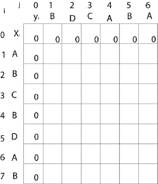
Now fill the values of c [i, j] in m x n table
Initially, for i=1 to 7 c [i, 0] = 0
For j = 0 to 6 c [0, j] = 0
That is:
|
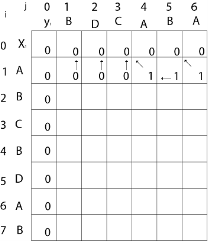
Now for i=1 and j = 1
x1 and y1 we get x1 ≠ y1 i.e. A ≠ B
And c [i-1,j] = c [0, 1] = 0
c [i, j-1] = c [1,0 ] = 0
That is, c [i-1,j]= c [i, j-1] so c [1, 1] = 0 and b [1, 1] = ' ↑ '
Now for i=1 and j = 2
x1 and y2 we get x1 ≠ y2 i.e. A ≠ D
c [i-1,j] = c [0, 2] = 0
c [i, j-1] = c [1,1 ] = 0
That is, c [i-1,j]= c [i, j-1] and c [1, 2] = 0 b [1, 2] = ' ↑ '
Now for i=1 and j = 3
x1 and y3 we get x1 ≠ y3 i.e. A ≠ C
c [i-1,j] = c [0, 3] = 0
c [i, j-1] = c [1,2 ] = 0
so c [1,3] = 0 b [1,3] = ' ↑ '
Now for i=1 and j = 4
x1 and y4 we get. x1=y4 i.e A = A
c [1,4] = c [1-1,4-1] + 1
= c [0, 3] + 1
= 0 + 1 = 1
c [1,4] = 1
b [1,4] = ' ↖ '
Now for i=1 and j = 5
x1 and y5 we get x1 ≠ y5
c [i-1,j] = c [0, 5] = 0
c [i, j-1] = c [1,4 ] = 1
Thus c [i, j-1] > c [i-1,j] i.e. c [1, 5] = c [i, j-1] = 1. So b [1, 5] = '←'
Now for i=1 and j = 6
x1 and y6 we get x1=y6
c [1, 6] = c [1-1,6-1] + 1
= c [0, 5] + 1 = 0 + 1 = 1
c [1,6] = 1
b [1,6] = ' ↖ '
|
Now for i=2 and j = 1
We get x2 and y1 B = B i.e. x2= y1
c [2,1] = c [2-1,1-1] + 1
= c [1, 0] + 1
= 0 + 1 = 1
c [2, 1] = 1 and b [2, 1] = ' ↖ '
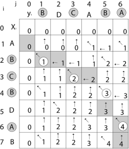
Similarly, we fill the all values of c [i, j] and we get
|
Step 4: Constructing an LCS: The initial call is PRINT-LCS (b, X, X.length, Y.length)
PRINT-LCS (b, x, i, j)
1. if i=0 or j=0
2. then return
3. if b [i,j] = ' ↖ '
4. then PRINT-LCS (b,x,i-1,j-1)
5. print x_i
6. else if b [i,j] = ' ↑ '
7. then PRINT-LCS (b,X,i-1,j)
8. else PRINT-LCS (b,X,i,j-1)
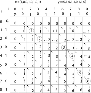
Example: Determine the LCS of (1,0,0,1,0,1,0,1) and (0,1,0,1,1,0,1,1,0).
Solution: let X = (1,0,0,1,0,1,0,1) and Y = (0,1,0,1,1,0,1,1,0).
|
We are looking for c [8, 9]. The following table is built.
|
From the table we can deduct that LCS = 6. There are several such sequences, for instance (1,0,0,1,1,0) (0,1,0,1,0,1) and (0,0,1,1,0,1)
Knapsack is basically means bag. A bag of given capacity.
We want to pack n items in your luggage.
- The ith item is worth vi dollars and weight wi pounds.
- Take as valuable a load as possible, but cannot exceed W pounds.
- vi wi W are integers.
- W ≤ capacity
- Value ← Max
Input:
- Knapsack of capacity
- List (Array) of weight and their corresponding value.
Output: To maximize profit and minimize weight in capacity.
The knapsack problem where we have to pack the knapsack with maximum value in such a manner that the total weight of the items should not be greater than the capacity of the knapsack.
Knapsack problem can be further divided into two parts:
1. Fractional Knapsack: Fractional knapsack problem can be solved by Greedy Strategy where as 0 /1 problem is not.
It cannot be solved by Dynamic Programming Approach.
In this item cannot be broken which means thief should take the item as a whole or should leave it. That's why it is called 0/1 knapsack Problem.
- Each item is taken or not taken.
- Cannot take a fractional amount of an item taken or take an item more than once.
- It cannot be solved by the Greedy Approach because it is enable to fill the knapsack to capacity.
- Greedy Approach doesn't ensure an Optimal Solution.
Example of 0/1 Knapsack Problem:
Example: The maximum weight the knapsack can hold is W is 11. There are five items to choose from. Their weights and values are presented in the following table:
|
The [i, j] entry here will be V [i, j], the best value obtainable using the first "i" rows of items if the maximum capacity were j. We begin by initialization and first row.
|
V [i, j] = max {V [i - 1, j], vi + V [i - 1, j -wi]
|
The value of V [3, 7] was computed as follows:
V [3, 7] = max {V [3 - 1, 7], v3 + V [3 - 1, 7 - w3]
= max {V [2, 7], 18 + V [2, 7 - 5]}
= max {7, 18 + 6}
= 24
|
Finally, the output is:
|
The maximum value of items in the knapsack is 40, the bottom-right entry). The dynamic programming approach can now be coded as the following algorithm:
KNAPSACK (n, W)
1. for w = 0, W
2. do V [0,w] ← 0
3. for i=0, n
4. do V [i, 0] ← 0
5. for w = 0, W
6. do if (wi≤ w & vi + V [i-1, w - wi]> V [i -1,W])
7. then V [i, W] ← vi + V [i - 1, w - wi]
8. else V [i, W] ← V [i - 1, w]
In the traveling salesman Problem, a salesman must visits n cities. We can say that salesman wishes to make a tour or Hamiltonian cycle, visiting each city exactly once and finishing at the city he starts from. There is a non-negative cost c (i, j) to travel from the city i to city j. The goal is to find a tour of minimum cost. We assume that every two cities are connected. Such problems are called Traveling-salesman problem (TSP).
We can model the cities as a complete graph of n vertices, where each vertex represents a city.
It can be shown that TSP is NPC.
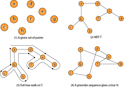
If we assume the cost function c satisfies the triangle inequality, then we can use the following approximate algorithm.
Let u, v, w be any three vertices, we have
|
One important observation to develop an approximate solution is if we remove an edge from H*, the tour becomes a spanning tree.
- Approx-TSP (G= (V, E))
- {
- 1. Compute a MST T of G;
- 2. Select any vertex r is the root of the tree;
- 3. Let L be the list of vertices visited in a preorder tree walk of T;
- 4. Return the Hamiltonian cycle H that visits the vertices in the order L;
- }
Traveling-salesman Problem
|
Fig 11 - Traveling-salesman Problem
Intuitively, Approx-TSP first makes a full walk of MST T, which visits each edge exactly two times. To create a Hamiltonian cycle from the full walk, it bypasses some vertices (which corresponds to making a shortcut)
A rod is given of length n. Another table is also provided, which contains different size and price for each size. Determine the maximum price by cutting the rod and selling them in the market.
To get the best price by making a cut at different positions and comparing the prices after cutting the rod.
Let the f(n) will return the max possible price after cutting a row with length n. We can simply write the function f(n) like this.
f(n) := maximum value from price[i]+f(n – i – 1), where i is in range 0 to (n – 1).
Input:
The price of different lengths, and the length of rod. Here the length is 8.
|
Output:
Maximum profit after selling is 22.
Cut the rod in length 2 and 6. The profit is 5 + 17 = 22
rodCutting(price, n)
Input: Price list, number of different prices on the list.
Output: Maximum profit by cutting rods.
Begin define profit array of size n + 1 profit[0] := 0 for i := 1 to n, do maxProfit := - ∞ for j := 0 to i-1, do maxProfit := maximum of maxProfit and (price[j] + profit[i-j-1]) done
profit[i] := maxProfit done return maxProfit End #include <iostream> using namespace std;
int max(int a, int b) { return (a > b)? a : b; }
int rodCutting(int price[], int n) { //from price and length of n, find max profit int profit[n+1]; profit[0] = 0; int maxProfit;
for (int i = 1; i<=n; i++) { maxProfit = INT_MIN; //initially set as -ve infinity for (int j = 0; j < i; j++) maxProfit = max(maxProfit, price[j] + profit[i-j-1]); profit[i] = maxProfit; } return maxProfit; }
int main() { int priceList[] = {1, 5, 8, 9, 10, 17, 17, 20}; int rodLength = 8; cout << "Maximum Price: "<< rodCutting(priceList, rodLength); }
|
Maximum Price: 22
Bin Packing Problem (Minimize number of used Bins)
In case of given m elements of different weights and bins each of capacity C, assign each element to a bin so that number of total implemented bins is minimized. Assumption should be that all elements have weights less than bin capacity.
- Placing data on multiple disks.
- Loading of containers like trucks.
- Packing advertisements in fixed length radio/TV station breaks.
- Job scheduling.
Input: weight[] = {4, 1, 8, 1, 4, 2}
Bin Capacity c = 10
Output: 2
We require at least 2 bins to accommodate all elements
First bin consists {4, 4, 2} and second bin {8, 2}
We can always calculate a lower bound on minimum number of bins required using ceil() function. The lower bound can be given below −
- Bins with minimum number >= ceil ((Total Weight) / (Bin Capacity))
- In the above example, lower bound for first example is “ceil(4 + 1 + 8 + 2 + 4 + 1)/10” = 2
- The following approximate algorithms are implemented for this problem.
These algorithms are implemented for Bin Packing problems where elements arrive one at a time (in unknown order), each must be put in a bin, before considering the next element.
Next Fit −
When processing next element, verify if it fits in the same bin as the last element. Implement a new bin only if it does not.
Following is C++ application for this algorithm.
// C++ program to calculate number of bins required implementing next fit algorithm. #include <bits/stdc++.h> using namespace std; // We have to return number of bins needed implementing next fit online algorithm int nextFit(int weight1[], int m, int C){ // Result (Count of bins) and remaining capacity in current bin are initialized. int res = 0, bin_rem = C; // We have to place elements one by one for (int i = 0; i < m; i++) { // If this element can't fit in current bin if (weight1[i] > bin_rem) { res++; // Use a new bin bin_rem = C - weight1[i]; } else bin_rem -= weight1[i]; } return res; } // Driver program int main(){ int weight1[] = { 3, 6, 5, 8, 2, 4, 9 }; int C = 10; int m = sizeof(weight1) / sizeof(weight1[0]); cout<< "Number of bins required in Next Fit : " <<nextFit(weight1, m, C); return 0; }
|
Number of bins required in Next Fit : 4
Next Fit is treated as a simple algorithm. It needs only O(m) time and O(1) extra space to process m elements.
First Fit−
When processing the next element, examine or scan the previous bins in order and place the element in the first bin that fits.If element does not fit in any of the existing bins at that time we start a new bin only.
// C++ program to find number of bins needed implementing First Fit algorithm. #include <bits/stdc++.h> using namespace std; // We have to return number of bins needed implementing first fit online algorithm int firstFit(int weight1[], int m, int C){ // We have to initialize result (Count of bins) int res = 0; // We have to create an array to store remaining space in bins there can be maximum n bins int bin_rem[m]; // We have to place elements one by one for (int i = 0; i < m; i++) { // We have to find the first bin that can accommodate weight1[i] int j; for (j = 0; j < res; j++) { if (bin_rem[j] >= weight1[i]) { bin_rem[j] = bin_rem[j] - weight1[i]; break; } } // If no bin could accommodate weight1[i] if (j == res) { bin_rem[res] = C - weight1[i]; res++; } } return res; } // Driver program int main(){ int weight1[] = { 2, 5, 4, 7, 1, 3, 8 }; int C = 10; int m = sizeof(weight1) / sizeof(weight1[0]); cout<< "Number of bins required in First Fit : " <<firstFit(weight1, m, C); return 0; }
|
Number of bins required in First Fit : 4
The above implementation of First Fit consumes O(m2) time, but First Fit can be used in O(m log m) time implementing Self-Balancing Binary Search Trees.
Best Fit −
The concept is to places the next item in the tightest position. That means put it in the bin so that at least emptyspace is left.
// C++ program to calculate number of bins required implementing Best fit algorithm.
#include <bits/stdc++.h>
using namespace std;
// We have to returns number of bins required implementing best fit online algorithm
int bestFit(int weight1[], int m, int C){
// We have to initialize result (Count of bins)
int res = 0;
// We have to create an array to store remaining space in bins there can be maximum n bins
int bin_rem[m];
// Place elements one by one
for (int i = 0; i < m; i++){
// Find the best bin that can accomodate weight1[i]
int j;
// We have to initialize minimum space left and index of best bin
int min = C + 1, bi = 0;
for (j = 0; j < res; j++){
if (bin_rem[j] >= weight1[i] && bin_rem[j] - weight1[i] < min) {
bi = j;
min = bin_rem[j] - weight1[i];
}
}
// We create a new bin,if no bin could accommodate weight1[i],
if (min == C + 1) {
bin_rem[res] = C - weight1[i];
res++;
}
else // Assign the element to best bin
bin_rem[bi] -= weight1[i];
}
return res;
}
// Driver program
int main(){
int weight1[] = { 2, 5, 4, 7, 1, 3, 8 };
int C = 10;
int m = sizeof(weight1) / sizeof(weight1[0]);
cout<< "Number of bins required in Best Fit : "
<<bestFit(weight1, m, C);
return 0;
}
Number of bins required in Best Fit : 4
Best Fit can also be applied in O(m log m) time implementing Self-Balancing Binary Search Trees.
In case of the offline version, we have all elements upfront.A problem with online algorithms is that packing large elements is difficult, especially if they occur late in the sequence. We can overcome this by sorting the input sequence, and placing the large elements first.
First Fit Decreasing −
// C++ program to locate number of bins needed implementing First Fit Decreasing algorithm.
#include <bits/stdc++.h>
using namespace std;
/* We copy firstFit() from above */
int firstFit(int weight1[], int m, int C){
// We have to initialize result (Count of bins)
int res = 0;
// We have to create an array to store remaining space in bins there can be maximum n bins
int bin_rem[m];
// We have to place elements one by one
for (int i = 0; i < m; i++) {
// We have to find the first bin that can accommodate weight1[i]
int j;
for (j = 0; j < res; j++) {
if (bin_rem[j] >= weight1[i]) {
bin_rem[j] = bin_rem[j] - weight1[i];
break;
}
}
// If no bin could accommodate weight1[i]
if (j == res) {
bin_rem[res] = C - weight1[i];
res++;
}
}
return res;
}
// We have to returns number of bins required implementing first fit decreasing offline algorithm
int firstFitDec(int weight1[], int m, int C){
// At first we sort all weights in decreasing order
sort(weight1, weight1 + m, std::greater<int>());
// Now we call first fit for sorted items
return firstFit(weight1, m, C);
}
// Driver program
int main(){
int weight1[] = { 2, 5, 4, 7, 1, 3, 8 };
int C = 10;
int m = sizeof(weight1) / sizeof(weight1[0]);
cout<< "Number of bins required in First Fit "
<< "Decreasing : " << firstFitDec(weight1, m, C);
return 0;
}
Number of bins required in First Fit Decreasing : 3
First Fit decreasing generates the best result for the sample input as elements are sorted first.
First Fit Decreasing can also be used in O(m log m) time implementing Self-Balancing Binary Search Trees.
C++ Program to Implement the Bin Packing Algorithm
The bin packing problem is a special type of cutting stock problem. In the bin packing problem, objects of different volumes must be packed into a finite number of containers or bins each of volume V in a way that minimizes the number of bins used. In computational complexity theory, it is a combinational NP-hard problem.
When the number of bins is restricted to 1 and each item is characterized by both a volume and a value, the problem of maximizing the value of items that can fit in the bin is known as the knapsack problem.
Begin
Binpacking(pointer, size, no of sets)
Declare bincount, m, i
Initialize bincount = 1, m=size
For i = 0 to number of sets
if (m - *(a + i) > 0) do
m = m - *(a + i)
Continue
Else
Increase bincount
m = size;
Decrement i
Print number of bins required
End
#include<iostream>
using namespace std;
void binPacking(int *a, int size, int n) {
int binCount = 1;
int m = size;
for (int i = 0; i < n; i++) {
if (m - *(a + i) > 0) {
m -= *(a + i);
continue;
} else {
binCount++;
m = size;
i--;
}
}
cout << "Number of bins required: " << binCount;
}
int main(int argc, char **argv) {
cout << "Enter the number of items in Set: ";
int n;
cin >> n;
cout << "Enter " << n << " items:";
int a[n];
for (int i = 0; i < n; i++)
cin >> a[i];
cout << "Enter the bin size: ";
int size;
cin >> size;
binPacking(a, size, n);
}
Enter the number of items in Set: 3
Enter 3 items:4
6
7
Enter the bin size: 26
Number of bins required: 1
Key takeaway
Fibonacci sequence is the sequence of numbers in which every next item is the total of the previous two items. And each number of the Fibonacci sequence is called Fibonacci number.
Longest Common Sequence (LCS)
A subsequence of a given sequence is just the given sequence with some elements left out.
Given two sequences X and Y, we say that the sequence Z is a common sequence of X and Y if Z is a subsequence of both X and Y.
In the longest common subsequence problem, we are given two sequences X = (x1 x2....xm) and Y = (y1 y2 yn) and wish to find a maximum length common subsequence of X and Y. LCS Problem can be solved using dynamic programming.
Traveling-salesman Problem
In the traveling salesman Problem, a salesman must visits n cities. We can say that salesman wishes to make a tour or Hamiltonian cycle, visiting each city exactly once and finishing at the city he starts from. There is a non-negative cost c (i, j) to travel from the city i to city j. The goal is to find a tour of minimum cost. We assume that every two cities are connected. Such problems are called Traveling-salesman problem (TSP).
Rod Cutting
A rod is given of length n. Another table is also provided, which contains different size and price for each size. Determine the maximum price by cutting the rod and selling them in the market.
To get the best price by making a cut at different positions and comparing the prices after cutting the rod.
Let the f(n) will return the max possible price after cutting a row with length n. We can simply write the function f(n) like this.
f(n) := maximum value from price[i]+f(n – i – 1), where i is in range 0 to (n – 1).
Bin Packing Problem (Minimize number of used Bins)
In case of given m elements of different weights and bins each of capacity C, assign each element to a bin so that number of total implemented bins is minimized. Assumption should be that all elements have weights less than bin capacity.
Applications
Placing data on multiple disks.
Loading of containers like trucks.
Packing advertisements in fixed length radio/TV station breaks.
Job scheduling.
The informed search algorithm is more useful for large search space. Informed search algorithm uses the idea of heuristic, so it is also called Heuristic search.
Heuristics function: Heuristic is a function which is used in Informed Search, and it finds the most promising path. It takes the current state of the agent as its input and produces the estimation of how close agent is from the goal. The heuristic method, however, might not always give the best solution, but it guaranteed to find a good solution in reasonable time. Heuristic function estimates how close a state is to the goal. It is represented by h(n), and it calculates the cost of an optimal path between the pair of states. The value of the heuristic function is always positive.
Admissibility of the heuristic function is given as:
- h(n) <= h*(n)
Here h(n) is heuristic cost, and h*(n) is the estimated cost. Hence heuristic cost should be less than or equal to the estimated cost.
Pure heuristic search is the simplest form of heuristic search algorithms. It expands nodes based on their heuristic value h(n). It maintains two lists, OPEN and CLOSED list. In the CLOSED list, it places those nodes which have already expanded and in the OPEN list, it places nodes which have yet not been expanded.
On each iteration, each node n with the lowest heuristic value is expanded and generates all its successors and n is placed to the closed list. The algorithm continues unit a goal state is found.
In the informed search we will discuss two main algorithms which are given below:
- Best First Search Algorithm(Greedy search)
- A* Search Algorithm
1.) Best-first Search Algorithm (Greedy Search):
Greedy best-first search algorithm always selects the path which appears best at that moment. It is the combination of depth-first search and breadth-first search algorithms. It uses the heuristic function and search. Best-first search allows us to take the advantages of both algorithms. With the help of best-first search, at each step, we can choose the most promising node. In the best first search algorithm, we expand the node which is closest to the goal node and the closest cost is estimated by heuristic function, i.e.
- f(n)= g(n).
Were, h(n)= estimated cost from node n to the goal.
The greedy best first algorithm is implemented by the priority queue.
- Step 1: Place the starting node into the OPEN list.
- Step 2: If the OPEN list is empty, Stop and return failure.
- Step 3: Remove the node n, from the OPEN list which has the lowest value of h(n), and places it in the CLOSED list.
- Step 4: Expand the node n, and generate the successors of node n.
- Step 5: Check each successor of node n, and find whether any node is a goal node or not. If any successor node is goal node, then return success and terminate the search, else proceed to Step 6.
- Step 6: For each successor node, algorithm checks for evaluation function f(n), and then check if the node has been in either OPEN or CLOSED list. If the node has not been in both list, then add it to the OPEN list.
- Step 7: Return to Step 2.
- Best first search can switch between BFS and DFS by gaining the advantages of both the algorithms.
- This algorithm is more efficient than BFS and DFS algorithms.
- It can behave as an unguided depth-first search in the worst case scenario.
- It can get stuck in a loop as DFS.
- This algorithm is not optimal.
Consider the below search problem, and we will traverse it using greedy best-first search. At each iteration, each node is expanded using evaluation function f(n)=h(n) , which is given in the below table.
|
In this search example, we are using two lists which are OPEN and CLOSED Lists. Following are the iteration for traversing the above example.
|
Expand the nodes of S and put in the CLOSED list
Initialization: Open [A, B], Closed [S]
Iteration 1: Open [A], Closed [S, B]
Iteration 2: Open [E, F, A], Closed [S, B]
: Open [E, A], Closed [S, B, F]
Iteration 3: Open [I, G, E, A], Closed [S, B, F]
: Open [I, E, A], Closed [S, B, F, G]
Hence the final solution path will be: S----> B----->F----> G
Time Complexity: The worst case time complexity of Greedy best first search is O(bm).
Space Complexity: The worst case space complexity of Greedy best first search is O(bm). Where, m is the maximum depth of the search space.
Complete: Greedy best-first search is also incomplete, even if the given state space is finite.
Optimal: Greedy best first search algorithm is not optimal.
A* search is the most commonly known form of best-first search. It uses heuristic function h(n), and cost to reach the node n from the start state g(n). It has combined features of UCS and greedy best-first search, by which it solve the problem efficiently. A* search algorithm finds the shortest path through the search space using the heuristic function. This search algorithm expands less search tree and provides optimal result faster. A* algorithm is similar to UCS except that it uses g(n)+h(n) instead of g(n).
In A* search algorithm, we use search heuristic as well as the cost to reach the node. Hence we can combine both costs as following, and this sum is called as a fitness number.
|
At each point in the search space, only those node is expanded which have the lowest value of f(n), and the algorithm terminates when the goal node is found.
Step1: Place the starting node in the OPEN list.
Step 2: Check if the OPEN list is empty or not, if the list is empty then return failure and stops.
Step 3: Select the node from the OPEN list which has the smallest value of evaluation function (g+h), if node n is goal node then return success and stop, otherwise
Step 4: Expand node n and generate all of its successors, and put n into the closed list. For each successor n', check whether n' is already in the OPEN or CLOSED list, if not then compute evaluation function for n' and place into Open list.
Step 5: Else if node n' is already in OPEN and CLOSED, then it should be attached to the back pointer which reflects the lowest g(n') value.
Step 6: Return to Step 2.
- A* search algorithm is the best algorithm than other search algorithms.
- A* search algorithm is optimal and complete.
- This algorithm can solve very complex problems.
- It does not always produce the shortest path as it mostly based on heuristics and approximation.
- A* search algorithm has some complexity issues.
- The main drawback of A* is memory requirement as it keeps all generated nodes in the memory, so it is not practical for various large-scale problems.
In this example, we will traverse the given graph using the A* algorithm. The heuristic value of all states is given in the below table so we will calculate the f(n) of each state using the formula f(n)= g(n) + h(n), where g(n) is the cost to reach any node from start state.
Here we will use OPEN and CLOSED list.
|
Solution:
|
Initialization: {(S, 5)}
Iteration1: {(S--> A, 4), (S-->G, 10)}
Iteration2: {(S--> A-->C, 4), (S--> A-->B, 7), (S-->G, 10)}
Iteration3: {(S--> A-->C--->G, 6), (S--> A-->C--->D, 11), (S--> A-->B, 7), (S-->G, 10)}
Iteration 4 will give the final result, as S--->A--->C--->G it provides the optimal path with cost 6.
Points to remember:
- A* algorithm returns the path which occurred first, and it does not search for all remaining paths.
- The efficiency of A* algorithm depends on the quality of heuristic.
- A* algorithm expands all nodes which satisfy the condition f(n) <="" li="">
Complete: A* algorithm is complete as long as:
- Branching factor is finite.
- Cost at every action is fixed.
Optimal: A* search algorithm is optimal if it follows below two conditions:
- Admissible: the first condition requires for optimality is that h(n) should be an admissible heuristic for A* tree search. An admissible heuristic is optimistic in nature.
- Consistency: Second required condition is consistency for only A* graph-search.
If the heuristic function is admissible, then A* tree search will always find the least cost path.
Time Complexity: The time complexity of A* search algorithm depends on heuristic function, and the number of nodes expanded is exponential to the depth of solution d. So the time complexity is O(b^d), where b is the branching factor.
Space Complexity: The space complexity of A* search algorithm is O(b^d)
Key takeaway
Heuristics function: Heuristic is a function which is used in Informed Search, and it finds the most promising path. It takes the current state of the agent as its input and produces the estimation of how close agent is from the goal. The heuristic method, however, might not always give the best solution, but it guaranteed to find a good solution in reasonable time. Heuristic function estimates how close a state is to the goal. It is represented by h(n), and it calculates the cost of an optimal path between the pair of states. The value of the heuristic function is always positive.
Reference:
1. Algorithm Design, 1st Edition, Jon Kleinberg and Éva Tardos, Pearson.
2. Algorithm Design: Foundations, Analysis, and Internet Examples, Second Edition, Michael T Goodrich and Roberto Tamassia, Wiley.
3. Algorithms—A Creative Approach, 3RD Edition, UdiManber, Addison-Wesley, Reading, MA.

