Unit - 5
Frequency domain analysis-II
In polar plot any point gives the magnitude phase of the transfer function in bode we split magnitude and  plot.
plot.
Advantages
By looking at bode plot we can write the transfer function of system
Q. G(S) = 
Substitute S = j
G(j ) =
) = 
M = 
 = tan-1
 = -900
Magnitude varies with ‘w’ but phase is constant.
MdB = +20 log10
MdB = -20 log10
Decade frequency:
W present = 10  past
past
Then  present is called decade frequency of
  past
past
 2 = 10
  1
1
 2 is decade frequency of
  1
1
 MdB
MdB
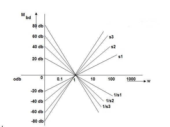
0.01 40
0.1 20
1 0 (shows pole at origin)
0 -20
10 -40
100 -60
Slope = (20db/decade)
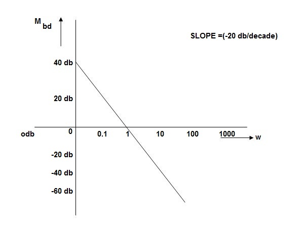
MAGNITUDE PLOT
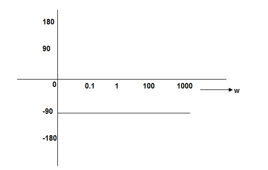
PHASE PLOT
Q.G(S) = 
G(j ) =
) = 
M =  ;
;  = -1800 (-20tan-1
 )
)
MdB = +20 log  -2
-2
MdB = -40 log10
 MdB
MdB
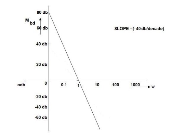
0.01 80
0.1 40
1 0 (pole at origin)
10 -40
100 -80
Slope = 40dbdecade
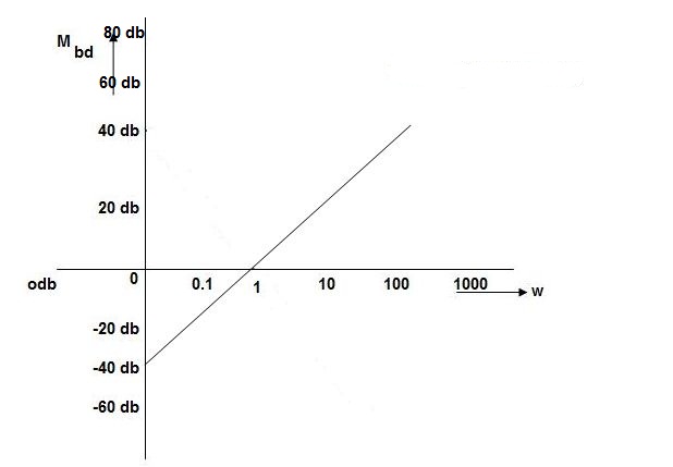
Q. G(S) = S
M= W
 = 900
= 900
MdB = 20 log10
 MdB
MdB
0.01 -40
0.1 -20
1 0
10 20
100 90
1000 60
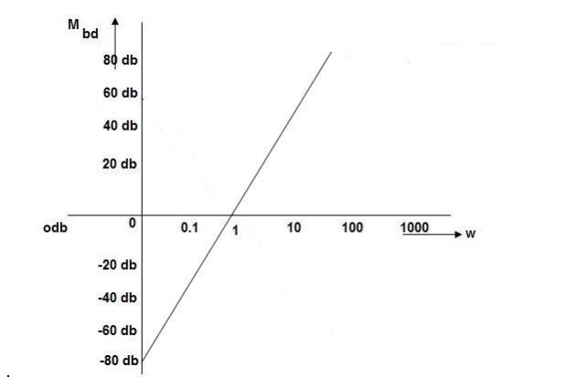
Q. G(S) = S2
M=  2 MdB = 20 log10
 2
2
 = 1800 = 40 log10
W MdB
0.01 -80
0.1 -40
1 0
10 40
100 80
Q. (S) = 
G(j ) =
) = 
M = 
MdB = 20 log10 K-20 log10
 = tan-1(
 ) –tan-1(
 )
)
 = 0-900 = -900
K=1 K=10  =-20 log10   0.01 40 60 0.1 20 40 1 0 20 10 -20 0 100 -40 -20 |
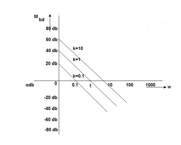
As we vary K  then plot shift by 20 log10K
i.e adding a d.c. To a.c. Quantity
IF poles and zeros are not located at origin
G(S) = 
TF = 
M = 
MdB = -20 log10 (
 = -tan-1
Approximation:  T >> 1. So, we can neglect 1.
MdB = -20 log10
MdB = -20 log10 T . ;
T . ;  = -tan-1(
 T)
T)
Approximation:  T << 1. So, we can neglecting
  T.
T.
MdB= 0dB,  = 00
= 00
At a point both meet so equal i.e a time will come hence both approx become equal
-20 log10 T= 0
T= 0
 T= 1
T= 1
 corner frequency
At this frequency both the cases are equal
MdB = -20 log10
Now for 
MdB = -20 log10
= -20 log10
= -10 log102
MdB = 10
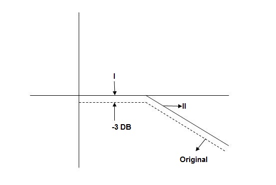
When we increase the value of  in app 2 and decrease the
  of app 1 so a RT comes when both cases are equal and hence for that value of
  where both app are equal gives max. Error we found above and is equal to 3dB
At corner frequency we have max error of -3dB
Q. G(S) = 
TF = 
M = 
MdB = -20 log10 ( at T=2
 MdB
MdB
1 -20 log10
10 -20 log10
100 -20 log10
 MdB
MdB  =
= =
= 
0.1 -20 log10 = 1.73
  10-3
10-3
0.1 -20 log10 = -0.1703
0.5 -20 log10 = -3dB
1 -20 log10 = -6.98
10 -20 log10 = -26.03
100 -20 log10 = -46.02

Without approximation
For second order system
TF = 
TF = 
= 
= 
= 
M= 
MdB= 
Case 1  <<
<<
 << 1
<< 1
MdB= 20 log10 = 0 dB
Case 2  >>
>>
 >> 1
>> 1
MdB = -20 log10
= -20 log10
= -20 log10
 < 1
< 1  is very large so neglecting other two terms
MdB = -20 log10
= -40 log10
Case 3 . When case 1 is equal to case 2
-40 log10 = 0
= 0
 = 1
= 1

The natural frequency is our corner frequency
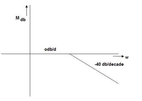
Max error at  i.e at corner frequency
MdB = -20 log10
For 
MdB = -20 log10 
 error for
Completely the error depends upon the value of  (error at corner frequency)
The maximum error will be
MdB = -20 log10 
M = -20 log10 
 = 0
= 0

 is resonant frequency and at this frequency we are getting the maximum error so the magnitude will be
M = - +
+ 
= 
Mr =
MdB = -20 log10
MdB = -20 log10 
 = tan-1

Mr = 
Type of system | Initial slope | Intersection |
0 | 0 dB/decade | Parallel to 0 axis |
1 | -20 dB/decade | =K1 |
2 | -40 dB/decade | =K1/2 |
3 | -60 dB/decade | =K1/3 |
. | . | 1 |
. | . | 1 |
. | . | 1 |
N | -20N dB/decade | =K1/N |
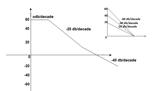
Q.1 sketch the bode plot for transfer function
G(S) = 
- Replace S = j

G(j =
= 
This is type 0 system. So initial slope is 0 dB decade. The starting point is given as
20 log10 K = 20 log10 1000
= 60 dB
Corner frequency  1 =
1 =  = 10 rad/sec
 2 =
2 =  = 1000 rad/sec
Slope after  1 will be -20 dB/decade till second corner frequency i.e
  2 after
  2 the slope will be -40 dB/decade (-20+(-20)) as there are poles
2. For phase plot
 = tan-1 0.1
 - tan-1 0.001
For phase plot


100 -900
200 -9.450
300 -104.80
400 -110.360
500 -115.420
600 -120.00
700 -124.170
800 -127.940
900 -131.350
1000 -134.420
The plot is shown in figure.
Q.2 For the given transfer function determine
G(S) = 
Gain cross over frequency phase cross over frequency phase mergence and gain margin
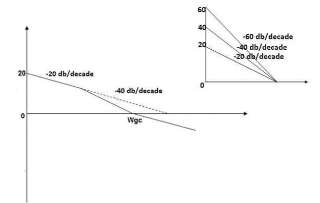
Initial slope = 1
N = 1, (K)1/N = 2
K = 2
Corner frequency
 1 =
1 =  = 2 (slope -20 dB/decade
 2 =
2 =  = 20 (slope -40 dB/decade

Phase
 = tan-1
 - tan-1 0.5
  - tan-1 0.05
 = 900- tan-1 0.5
  - tan-1 0.05


1 -119.430
5 -172.230
10 -195.250
15 -209.270
20 -219.30
25 -226.760
30 -232.490
35 -236.980
40 -240.570
45 -243.490
50 -245.910
Finding  gc (gain cross over frequency
M = 
4 =  2 (
2 ( (
(
 6 (6.25
 104) + 0.252
 4 +
4 + 2 = 4
2 = 4
Let  2 = x
2 = x
X3 (6.25 104) + 0.252
 2 + x = 4
X1 = 2.46
X2 = -399.9
X3 = -6.50
For x1 = 2.46
 gc = 3.99 rad/sec(from plot )
For phase margin
PM = 1800 - 
 = 900 – tan-1 (0.5×
 gc) – tan-1 (0.05 ×
  gc)
gc)
= -164.50
PM = 1800 - 164.50
= 15.50
For phase cross over frequency ( pc)
pc)
 = 900 – tan-1 (0.5
  ) – tan-1 (0.05
  )
)
-1800 = -900 – tan-1 (0.5  pc) – tan-1 (0.05
  pc)
pc)
-900 – tan-1 (0.5  pc) – tan-1 (0.05
  pc)
pc)
Taking than on both sides
Tan 900 = tan-1
Let tan-1 0.5  pc = A, tan-1 0.05
  pc = B
 = 00
= 00
 = 0
= 0
1 =0.5  pc 0.05
 pc
pc
 pc = 6.32 rad/sec
The plot is shown in figure below.
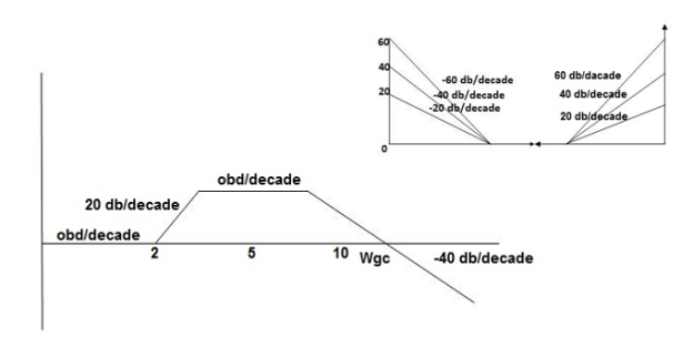
Q3. For the given transfer function
G(S) = 
Plot the rode plot find PM and GM
T1 = 0.5  1 =
1 =  = 2 rad/sec
Zero so, slope (20 dB/decade)
T2 = 0.2  2 =
2 =  = 5 rad/sec
Pole, so slope (-20 dB/decade)
T3 = 0.1 = T4 = 0.1
 3 =
3 =  4 = 10 (2 pole) (-40 db/decade)
- Initial slope 0 dB/decade till
 1 = 2 rad/sec
 - From
 1 to
1 to 2 (i.e. 2 rad /sec to 5 rad/sec) slope will be 20 dB/decade
 - From
 2 to
2 to  3 the slope will be 0 dB/decade (20 + (-20))
 - From
 3,
3, 4 the slope will be -40 dB/decade (0-20-20)
Phase plot
 = tan-1 0.5
 - tan-1 0.2
 - tan-1 0.1
 - tan-1 0.1


500 -177.30
1000 -178.60
1500 -179.10
2000 -179.40
2500 -179.50
3000 -179.530
3500 -179.60
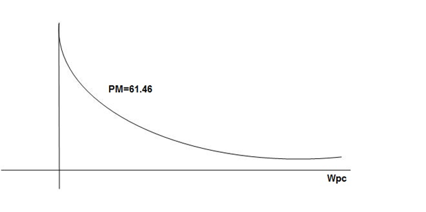
GM = 00
PM = 61.460
The plot is shown in figure
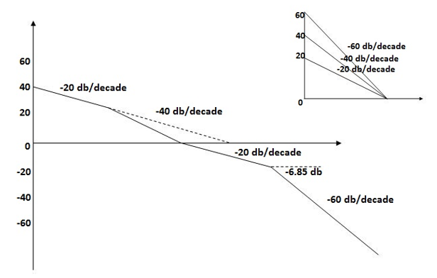
Q4. For the given transfer function plot the bode plot (magnitude plot)
G(S) = 
Given transfer function
G(S) = 
Converting above transfer function to standard from
G(S) = 
= 
1. As type 1 system, so initial slope will be -20 dB/decade
2. Final slope will be -60 dB/decade as order of system decides the final slope
3. Corner frequency
T1 =  ,
,  11= 5 (zero)
T2 = 1,  2 = 1 (pole)
4. Initial slope will cut zero dB axis at
(K)1/N = 10
i.e  = 10
= 10
5. Finding  n and
n and 
T(S) = 
T(S)= 
Comparing with standard second order system equation
S2+2 ns +
ns + n2
n2
 n = 11 rad/sec
 n = 5
n = 5
 11 = 5
 =
=  = 0.27
6. Maximum error
M = -20 log 2
= +6.5 dB
7. As K = 10, so whole plot will shift by 20 log 10 10 = 20 dB
The plot is shown in figure below.
Q5. For the given plot determine the transfer function
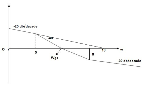
From above figure we can conclude that
1. Initial slope = -20 dB/decade so type -1
2. Initial slope alls 0 dB axis at  = 10 so
K1/N N = 1
(K)1/N = 10.
3. Corner frequency
 1 =
1 =  = 0.2 rad/sec
 2 =
2 =  = 0.125 rad/sec
4. At  = 5 the slope becomes -40 dB/decade, so there is a pole at
  = 5 as slope changes from -20 dB/decade to -40 dB/decade
5. At  = 8 the slope changes from -40 dB/decade to -20 dB/decade hence is a zero at
  = 8 (-40+(+20)=20)
6. Hence transfer function is
T(S) = 
Stability Condition in Bode Plot:
Gain Cross Over Frequency:
The frequency at which the bode plot culls the 0db axis is called as Gain Cross Over Frequency.

Phase Cross Over Frequency-:
The Frequency at which the phase plot culls the -1800 axis.
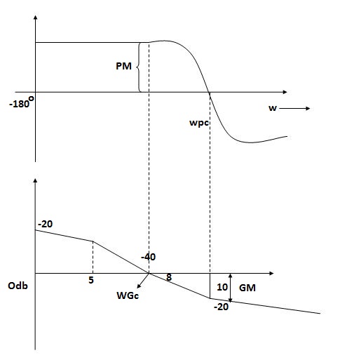
GM=MdB= -20 log [ G (jw)]
 .:
.: 
 .:
.: 
1) When gain cross over frequency is smaller than phase curves over frequency the system is stable and vice versa.
Inference1:
More the difference b/WPC and WGC core is the stability of system
Inference 2:
If GM is below 0dB axis than take ilb +ve and stable. If GM above 0dB axis , that is take -ve
GM= ODB - 20 log M * * L
Inference 3:
1) The IM should also lie above -1800 for making the system (i.e. pm=+ve
For a stable system GM and PM should be -ve
2)GM and PM both should be +ve more the value of GM and PM more the system is stable.
3)If Wpc and Wgc are in same line Wpc= Wgc than system is marginally stable as we get GM=0dB.
References:
1) B. C. Kuo, “Automatic Control System”, Wiley India, 8th Edition, 2003.
2) Richard C Dorf and Robert H Bishop, “Modern control system”, Pearson Education, 12th edition, 2011.
3) D. Roy Choudhary, "Modern Control Engineering", PHI Learning Pvt. Ltd., 2005.