Unit – 4

Basic Statistics

4.1 Measures of Central tendency: Moments, Skewness and Kurtosis

Average or Measures of Central tendency

An average is a value which is representative of a set of data. Average value may also be termed as measures of central tendency. There are five types may also be termed as measures of central tendency. There are five types of averages in common.

1. Arithmetic average or mean
2. Median
3. Mode
4. Geometric Mean
5. Harmonic Mean

Arithmetic Mean

If are n numbers, then their arithmetic mean (A.M) is defined by

If the number occurs times, occurs times and so on, then

This is known as direct method.

Example 1: Find the mean of 20, 22, 25, 28, 30.

Solution:

Example 2: Find the mean of the following:

Solution:

(b) Shortcut method

Let be the assumed mean, d the deviation of the variate from . Then

Example 3: Find the arithmetic mean for the following distribution:

Solution:

Let assumed mean

Class	Mid-value	Frequency
0-10 10-20 20-30 30-40 40-50	5 15 25 35 45	7 8 20 10 5	-20 -10 0 10 5	-140 -80 0 100 100
Total			50	-20

(c) Step deviation method

Letbe the assumed mean, the width of the class interval and

Median

Median is defined as the measure of the central item when they are arranged in ascending or descending order of magnitude.

When the total number of the items is odd and equal to say then there are two middle items, and so the mean of the values of and items is the median.

Example 5:

Find the median of

Solution:

Total number of items =7

The middle item

Median=Value of the 4th item=10

For grouped data, Median

Where is the lower limit of the median class, is the frequency of the class, is the width of the class- interval, F is the total of all the preceeding frequencies of the median – class and N is total frequency of the data.

Example 6:

Find the value of Median from the following data.

Solution: The given cumulative frequency distribution will first be converted into ordinary frequency as under

Class Interval	Cumulative frequency	Ordinary frequency
0-5 5-10 15-20 20-25 25-35 30-35 35-40 40-45	29 465 582 634 644 650 653 655	29=29 224-29=195 465-224= 582-465=117 634-582=52 644-634=10 650-644=6 653-650=3 655-653=2

Median= size of or 327.5th item

327.5th item lies in 10-15 which is the median class.

Where stands for lower limit of median class,

N stands for the total frequency,

C stands for the cumulative frequency just preceding the median class,

stands for class interval

stands for frequency for the median class.

Median

Mode

Mode is defined to be the size of the variable which occurs most frequently.

Example 7:

Find the mode of the following items:

0, 1, 6, 7, 2, 3, 7, 6, 6, 2, 6, 0, 5, 6, 0.

Solution:

6 occurs 5 times and no other item occurs 5 or more than 5 times, hence the mode is 6.

For grouped data,  Mode

Where is the lower limit of the modal class, is  the frequency of the modal class, is the width of the class, is the frequency before the modal class and of the frequency after the modal class.

Empirical formula

Mean – Mode = 3 [Mean – Median]

Example 8:

Find the mode from the following data:

Solution:

Age	Frequency	Cumulative frequency
0-6 6-12 12-18 24-30 30-36 36-42	6 11          25         35        12 6	6 17 42 77 95 107 113

Mode

Geometric Mean

If be n values of variates x, then the geometric mean

Example 10.

Calculate the harmonic mean of 4, 8, 16.

Solution:

Average deviation or Mean Deviation

It is the mean of the absolute values of the deviations of a given set of numbers from their arithmetic mean.

If be a set of numbers with frequencies respectively. Let be the arithmetic mean of the numbers ,then

Mean deviation

Example 11:

Find the mean deviation of the following frequency distribution.

Solution:

Let

Class	Mid value	Frequency
0-6 6-12 12-18 18-24 24-30	3 9 15 21 27	8 10 12 9 5	-12 -6 0 6 12	-96 -60 0 54 60	11 5 1 7 13	88 50 12 63 65
Total		44		-42		278

Mean

Average deviation

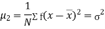
MOMENTS

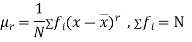
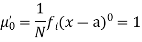
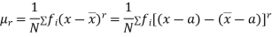
The rth moment of a variable x about the mean x is usually denoted by is given by

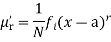
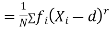
The rth moment of a variable x about any point a is defined by

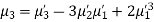
Relation between moments about mean and moment about any point:

where and

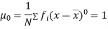
In particular

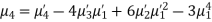
Note. 1. The sum of the coefficients of the various terms on the right‐hand side is zero.

2. The dimension of each term on right‐hand side is the same as that of terms on the left.

MOMENT GENERATING FUNCTION

The moment generating function of the variate about is defined as the expected value of and is denoted .

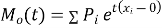
Where , ‘ is the moment of order about

Hence coefficient of or

Again )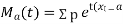

Thus, the moment generating function about the point moment generating function about the origin.

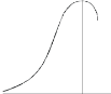
SKEWNESS:

Skewness denotes the opposite of symmetry. It is lack of symmetry. In a symmetrical series, the mode, the median, and the arithmetic average are identical.

Coefficient of skewness

KURTOSIS: It measures the degree of peakedness of a distribution and is given by Measure of kurtosis.

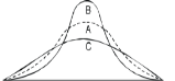
Negative skewness               Positive skewness              A: Mesokurtic B: Leptokurtic

C: Playkurtic

If , the curve is normal or mesokurtic.

If , the curve is peaked or leptokurtic.

If , the curve is flat topped or platykurtic

Example

The first four moments about the working mean 28.5 of  a distribution 0.294, 7.144, 42.409 and 454.98. Calculate the moments about the mean. Also evaluate and comment upon the skewness and kurtosis of the distribution.

Solution:

The first four moments about the arbitrary origin 28.5 are, , and .

    or

Now 

  which indicates considerable skewness of the distribution.

which shows that the distribution is leptokurtic.

Example

Calculate the median, quartiles and the quartile coefficient of skewness from the following data:

Solution

Here total frequency .

The cumulative frequency table is

Weight (lbs)	70-80	80-90	90-100	100-110	110-120	120-130	130-140	140-150
	12	18	35	42	50	45	20	8
	12	30	65	107	157	202	222	230

Now item which lies in 110-120 group.

 Median or

Also i.e. is or item which lies in 90-100 group.

Similarly, i.e.,is item which lies in 120-130 group.

Hence quartile coefficient of skewness

(approx..)

4.2 Probability distributions – Binomial, Poisson and Normal: Evaluation of statistical parameters for these three distributions

A probability distribution is a arithmetical function which defines completely possible values &possibilities that a random variable can take in a given range. This range will be bounded between the minimum and maximum possible values. But exactly where the possible value is possible to be plotted on the probability distribution depends on a number of influences. These factors include the distribution's mean, SD, Skewness, and kurtosis.

Binomial Distribution:

Binomial Distribution

To find the probability of the happening of an event once, twice, …., r times… exactly in n trials.

Let the probability of the happening of an event A in one trial be and its probability of not happening be

We assume that there are n trials and the happening of the event a is r times and its not happening n-r times.

This may be shown as follows

r times   n-r times   ….(1)

A indicates its happening, its failure and and.

We see that (1) has the probability

   …. (2)

r times    n-r times

Clearly (1) is merely one order of arranging r A’s

The probability of (1) Number of different arrangements of and                                       .

The number of different arrangements of and

Probability off the happening of an event times

th term of

If , probability of happening of an event 0 times

If , probability of happening of an event 1 times

If , probability of happening of an event 2 times

If ,  probability of happening of an event 3 times

These terms are clearly the successive terms in the expansion of . Hence it is called Binomial distribution.

Example

If on an average one ship in every ten is wrecked, find the probability that of 5 ships expected to arrive, 4 at least will arrive safely.

Solution:

Out of 10 ships, one ship is wrecked.

i.e., Nine ships out of ten ships are safe. P(safety)

P(At least 4 ships out of 5 ships are safe)

Example

The overall percentage of failures in a certain examination is 20. If six candidates appear in the examination, what is the probability that at least five pass the examination?

Solution:

Probability of failures

Probability

Probability of at least five pass P(5 or 6)

Example

The probability that a man aged 60 will live to be 70 is 0.65. What is the probability that out of 10 item, now 60, at least 7 will live to be 70?

Solution

The probability that a man aged 60 will live to be 70

Number of men

Probability that at least 7 men will live to

Example

A die is thrown 8 times and it is required to find the probability that 3 will show (i) Exactly 2 times

(ii) At least seven times (iii) At least once.

Solution:

The probability of throwing 3 in a single trial =

The probability of not throwing 3 in a single trial

(i)  P (getting 3 exactly 2 times)=P (getting 3, at 7 or 8 times)

(ii)  P (getting 3, at least seven times)=P (getting 3, at 7 or 8 times)  

(iii) P (getting 3 at least once)

= P (getting 4, at 1 or 2 or 3 or 4 or 5 or 6 or 7 or 8 times)

Example:

Assuming that 20% of the population of a city are literate, so that the chance of an individual being literate is and assuming that 100 investigators each take 10 individuals to see whether they are literate, how many investigators would you expect 3 or less were literate.

Solution    

P (3 or less) = P (0 or 1 or 2 or 3 )

Required number of investigators

approximately

Mean of Binomial Distribution

Successes	Frequency
0
1
2
3
…	….	….
4

Hence  Mean

Standard Deviation of Binomial Distribution

Successes	Frequency
0
1
2
3
….	….	…
n

We know that    ….(1)

is the deviation of items (successes) from 0.

Putting these values in (1), we have

Variance

Hence for the binomial distribution, Mean

Example:

A die is tossed thrice. A success is getting 1 or 6 on a toss. Find the mean and variance of the number of successes.

Solution:

Mean

Variance

Recurrence relation for the binomial distribution

By Binomial distribution

On dividing (2) by (1), we get  

Poisson Distribution:

Poisson distribution is a particular limiting form of the Binomial distribution when p or (q) is very small and n is large enough.

Poisson distribution is

Where m is the mean of the distribution.

Proof:

In Binomial distribution

  { Since mean } 

  (m is constant)

Taking limits, when n tends to infinity

Mean of Poisson Distribution

Successes	Frequency
0		0
1
2
3
…	…	….
r
…	…	….

Mean  

Standard Deviation of Poisson Distribution

Successes	Frequency	Product	Product
0		0	0
1
2
3
…	….	….	…
r
…	….	…	…

Hence mean and variance of a Poisson distribution are each equal to m. Similarly we can obtain,

Mean Deviation:

Show that in a Poisson distribution with unit mean, and the mean deviation about the mean is times the standard deviation.

Solution:  But mean=1   i.e.,   and

Hence,   

0		1
1		0
2		1
3		2
4		4
…	….	….	…
r		r-1

Mean Derivation

Moment Generating Function of Poisson Distribution

Solution:

Let be the moment generating function, then

Cumulants

The cumulant generating function is given by

Now cumulant Coefficient of  in K(t)

i.e.,    where

Mean

Recurrence formula for Poisson Distribution:

Solution:  By Poisson Distribution

On dividing (2) by (1) we get

Example

Assume that the probability of on individual coal miner being killed in a mine accident during a year is. Use appropriate statistical distribution to calculate the probability that in a mine employing 200 metres, there will be at least one fatal accident in a year.

Solution:

,  

P(At least one)=P(1 or 2 or 3 or …. Or 200)

Example:

Suppose 3% of bolts made by a machine are defective, the defects occurring at random during production. If bolts are packaged 50 per box, find

(a) exact probability and

(b) Poisson approximation to it, that a given box will contain 5 defectives.

Solution:

(a) Hence the probability for 5 defective bolts in a lot of 50

  (Binomial Distribution)

(b) To get Poisson approximation

Required Poisson approximation

Example:

In a certain factory producing cycle tyres there is a  small chance of 1 in 500 tyres to be defective. The tyres are supplied in lots of 10. Using Poisson distribution calculate the approximate number of lots containing no defective, one defective and two defective tyres, respectively, in a consignment of 10000 lots.

Solution:

S.No	Probability of defective	Number of lots containing defective
1
2
3

Normal Distribution:

Normal distribution is a continuous distribution. It is derived a s the limiting form of the Binomial distribution for large values of n and p and q are not very small.

The Normal distribution is given by the equation

  ….(1)

Where mean, standard deviation, , 

On substitution in (1), we get  ….(2)

Here mean, standard deviation

(2) is known as standard form of normal distribution.

Mean for Normal Distribution:

Mean   [Putting ]

Standard Deviation for Normal Distribution:

Put 

Median of the Normal Distribution

If a is the median, then it divides the total area into two equal halves so that,

Where  

Suppose mean, then

  [But]

  (mean)

Thus    

Similarly, when mean, we have

Thus, median=median.

Mean Deviation about the Mean

Mean Deviation   

  where

  (as the function is given)

 approximately.

Mode of the Normal distribution

We know that mode is the value of the variate x for which is maximum. Thus, by differential calculus is maximum if and

Where

Clearly will be maximum when the exponent will bemaximum which will be the when

Thus mode is and modal ordinate

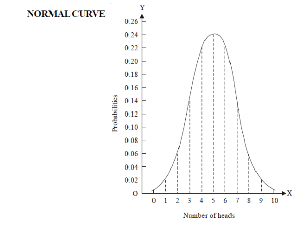
Let us show binomial distribution graphically. The probabilities of heads in 1 tosses are.

. It is shown in the given figure.

If the variates (heads here) are treated as if they were continuous, the required probability curve will be a normal curve as shown in the above figure by dotted lines.

Properties of the normal curve:

1. The curve is symmetrical about the y – axis. The mean, median and mode coincide at the origin.
2. The curve is drawn, if mean (origin of x) and standard deviation are given. The value of can be calculated from the fact that the area of the curve must be equal to the total number of observations.
3. Y decreases rapidly as increases numericallu. The curve extends to infinity on either side of the origin.
4. (a)        

(b)

(c) 

Hence (a) About of the values will lie between and .

(b) About 95% of the values will lie betweenand .

(c)  About 99.7% of the values will lie betweenand .

Area under the Normal curve

By taking , the standard normal curve is formed.

The total area under this curve is 1. The area under the curve is divided into two equal parts by. Left hand side are and right hand side area to is . The area between the ordinate.

Example

On final examination in mathematics, the mean was 72, and the standard deviation was 15. Determine the standard deviation scores of students receiving graders.

(a)  60   (b)  93   (c)  72

Solution:

(a)  (b)  (c) 

Example: Find the area under the normal curve in each of the cases.  

Solution:

(a) Area between and  (b) Area between and

(c) Required area (Area between and )+

(Area between and )

=( Area between and )

+( Area between and )  

(d) Required area (Area between and ) – (Area between                                                                              and )

(e) Required area(Area between and )  

(f) Required area = (Area between and )

Example. The mean inside diameter of a sample of 200 washers produced by a machine is 0.0502 cm and the standard derivation is 0.005 cm. The purpose for which these washers are intended allows a maximum tolerance in the diameter of 0.496 to 0.508 cm, otherwise the washers are considered defective. Determine the percentage of defective washers produced by the machine, assuming the diameters are normally distributed

Solution:

Area for non-defective washersArea between and

= 2 Area between and

Percentage of defective washers

Example:

A manufacturer knows from experience that the resistance of resistors he produces is normal with mean and standard deviation What percentage of resistors will have resistance between 98 ohms and 102 ohms?

Solution:

Area between and

( Area between and )+( Area between and )

( Area between and )=20.3413=0.6826

Percentage of resistors having resistance between 98 ohms and 102 ohms =68.26

Example

In a normal distribution, 31% of the items are under 45 and 8% are over 64. Find the mean and standard deviation of the distribution.

Solution:

Let be the mean and the S.D.

If

If

Area between 0 and

[From the table, for the area ]

   …(1)

Area between and

(From the table, for area)

   …(2)

Solving (1) and (2), we get

4.3 Correlation and regression – Rank correlation

Correlation

So far we have confined our attention to the analysis of observation on a single variable. There are , however, many phenomena where the changes in one variable are related to the changes in the other variable.  For instance, the yield of crop varies with the amount of rainfall, the price of a commodity increases with the reduction in its supply and so on. Such a simultaneous variation, i.e., when the changes in one variable are associated or followed by change in the other, is called correlation. Such a data connecting two variables is called bivariate population.

If an increase (or decrease) in the values of one variable corresponds to an increase (or decrease) in the other, the correlation is said to be positive. If the increase (or decrease) in one corresponds to the decrease (or increase) in other, the correlation is said to be negative.  If there is no relationship indicated between the variables, they are said to be independent or uncorrelated.

To obtain a measure of relationship between the two variable, we plot their corresponding values on the graph, taking one of the variables along the x-axis and the other along the y-axis (Fig 35.6).

Let the origin be shifted to, where are the means of x’s and y’s that the new co-ordinates are given by

,     

Now the points (X,Y) are so distributed over the four quadrants of XY –plane that the product XY is positive in the first and third quadrants but negative in the second and fourth quadrants. The algebraic sum of the products can be taken as describing the trend of the dots in all the quadrants.

 (i) Ifis possible the trend of the dots is through the first and third quadrants,

(ii) If is negative the trend of the dots is in the second and fourth quadrants, and

(iii) If is zero, the points indicate no trend i.e., the points are evenlu distributed over the four quadrants.             

Theor better still , i.e.,  the average of n products may be taken as a measure of correlation. If we put X and U in their units, i.e., taking as the unit for and for , then

Is the measure of correlation.

Coefficient of Correlation:

The numerical measure of correlation is called the coefficient of correlation and is defined by the relation

Where derivation from the mean ,

derivation from the mean

S.D of x – series, S.D of y-series and

number of values of the two variables.

Methods of calculation:

(a) Direct method. Substituting the value of andin the above formula, we get  

Another form of the formula (1) which is quite handy for calculation is

(b) Step deviation method. The direct method become very lengthy and tedious if the means of the two series are not integers. In such cases, use is made of assumed means. If and are step-deviation from the assumed means, then

Where and

Obs: The change of origin and units do not alter the value of the correlation coefficient since r is a pure number.

(c) Co-efficient of correlation for grouped data.  When x and y series ae both given as frequency distributions, these can be represented by a two-way table known as the correlation-table. The co-efficient of correlation for such a bivariate frequency distribution is calculated by the formula.

Where deviation of the central values from the assumed mean of x – series,

deviation of the central values fromt eh assumed mean of y-series,

is the frequency corresponding to the pair

is the total number of frequencies.

Example

Psychological tests of intelligence and of engineering ability were applied to 10 students. Here is a record of ungrouped data showing intelligence ratio (I.R) and engineering ratio (E.R). Calculate the co-efficient of correlation.

Solution:

We construct the following table:

Student	Intelligence ratio	Engineering ratio
A B C D E F G H I J	100                      6     104                     5     102                     3     101                     2     100                     1       99                     0       98                    -1       96                    -3       93                    -6       92                    -7	101                 3   103                 5   100                 2    98                  0    95                 -3    96                 -2   104                 6    92                 -6    97                 -1    94                 -4	36 25 9 4 1 0 1 9 36 49	9 25 4 0 9 4 36 36 1 16	18 25 6 0 -3 0 -6 18 6 28
Total	990                    0	980                 0	170	140	92

From this table, mean of i.e., and mean of , i.e.,

Substituting these values in the formula (1), we have

Example:

The correlation table given below shows that the ages of husband and wife of 53 married couples living together on the census night of 1991. Calculus the coefficient of correlation between the age of the husband and that of the wife.

Solution:

Age of husband				Age of wife - series							Suppose
				15-25	25-35	35-45	45-55	55-65	65-75	Total
Years			Mid Pt.	20	30	40	50	60	70
				-20	-10	0	10	20	30
Age Group	Mid Pt.			-2	-1	0	1	2	3
15-25	20	-20	-2							2	-4	8	6
25-35	30	-10	-1							15	-15	15	16
35-45	40	0	0							15	0	0	0
45-55	50	10	1							10	10	10	8
55-65	60	20	2							8	16	32	32
65-75	70	30	3							3	9	27	24
Total				3	17	14	9	6	4	53	16	92	86
				-6	-17	0	9	12	12	10	Thick figures in small squares Stand for Check: =86  from both sides
				12	17	0	9	24	36	98
				8	14	0	10	24	30	86

With the help of the above correlation table, we have

(approx.)

Line of Regression:

It frequently happens that the dots of the scatter diagram generally, tend to cluster along a well-defined direction which suggests a linear relationship between the variables and . Such a line of best-fit for the given distribution of dots is called the line of regression. (Fig 25.6). In fact there are two such lines, one giving the best possible mean values of . The former is known as the line of regression of y on x and the latter as the line of regression of x on y.

Consider first the line of regression of y on x. Let the straight line satisfying the general trend of n dots in a scatter diagram be

   …. (1)

We have to determine the constants a and b so that (1) gives for each value of x, the best estimate for the average value of y in accordance with the principle of least squares therefore, the normal equations for a and b are

   …. (2)

   …. (3)

(2) gives   

This shows that , i.e., the means of x and y, lie on (1).

Shifting the origin to, (3) takes the form

, but ,

Thus the line of best fit becomes    …. (4)  

Which is the equation of the line of regression of y on x. Its slope is called the regression coefficient of y on x.

Interchanging x and y, we find that the line of regression of x on y is

    …. (5)

Thus the regression coefficient of y on    …. (6)

And the regression coefficient of x on    …. (7)

Cor. The correlation coefficient is the geometric mean between the two regression co-efficients.

For   

Example

The two regression equations of the variables and areand . Find (i) mean of ’s (ii) mean of ’s and (iii) the correlation coefficient between and.

Solution:

Since the mean of ’s and the mean of’s lie on the two regression line, we have

Multiplying (ii) by 0.87 and subtracting from (i), we have

  Regression coefficient of y on x is -0.50 and that of x on y is -0.87.

Now the since coefficient of correlation is the geometric mean between the two regression coefficients.

[-ve sign is taken since both the regression coefficients are –ve]

Example.

If is the angle between the two regression lines, show that

Explain the significance when and .

Solution:

The equations to the line of regression of y on x and x on y are

and

 Their slopes areand

Thus    

When or i.e., when the variables are independent, the two lines of regression are perpendicular to each other.

When or . Thus the lines of regression coincide i.e, there is perfect correlation between the two variables.

Example:

In a partially destroyed laboratory record, only the lines of regression of y on x and x on y are available as and respectively. Calculate and the coefficient of correlation between x and y.

Solution:

Since the regression lines pass through, therefore,

,

Solving these equations, we get

Rewriting the line of regression of y on x as, we get

    …. (i)

Rewriting the line of regression of x on y as, we get

  …. (ii)

Multiplying (i) and (ii), we get

Hence , the positive sign being taken as and both are positive.

Example:

8 6	12 8

While calculating correlation coefficient between two variables x and y from 25 pairs of observations, the following result were obtained: ,. Later it was discovered at the time of checking that the pairs of values     were copied down as

6 8	14 6

Obtain the correct value of coefficient.

Solution:

To get the correct results, we subtract the incorrect values and add the corresponding correct values.

The correct results would be

Rank Correlation

A group of n individuals may be arranged in order to merit with respect to some characteristic. The same group would give different orders for different characteristics. Considering the order corresponding to two characteristics A and B for that group of individuals.

Let be the ranks of the ith individuals in A and B respectively. Assuming that no two individuals are bracketed equal in either case, each of the variables taking the values 1,2,3,…,n, we have

If X,Y be the deviation of x, y from their means, then

Similarly

Now let so that

Hence the correlation coefficient between these variables is

This is called the rank correlation coefficient and is denoted by.

Example:

	1	6	5	10	3	2	4	9	7	8
	6	4	9	8	1	2	3	10	5	7

Solution:

If   , then

Hencenearly.

Example

Three judges A, B, C, give the following ranks. Find which pair of judges has common approach

Solution: Here

	Ranks by
1 6 5 10 3 2 4 9 7 8	3 5 8 4 7 10 2 1 6 9	6 4 9 8 1 2 3 10 5 7	-2 1 -3 6 -4 -8 2 8 1 -1	-3 1 -1 -4 6 8 -1 -9 1 2	5 -2 4 -2 -2 0 -1 1 -2 -1	4 1 9 36 16 64 4 64 1 1	9 1 1 16 36 64 1 81 1 4	25 4 16 4 4 0 1 1 4 1
Total			0	0	0	200	214	60

Since is maximum, the pair of judges A and C have the nearest common approach.

Reference

1. Erwin Kreyszig, Advanced Engineering Mathematics, 9th Edition, John  Wiley and amp; Sons, 2006.
2. N.P. Bali and Manish Goyal, A text book of Engineering Mathematics,  Laxmi Publications, Reprint, 2010.
3. Veerarajan T., Engineering Mathematics (for semester III), Tata McGraw- Hill, New Delhi, 2010
4. C. L. Liu, Elements of Discrete Mathematics, 2nd Ed., Tata McGraw-Hill, 2000.