Unit – 2 | unit 2 system modelling in terms of differential equations

Back to Study material

Network Theory

Unit – 2

System modelling in terms of differential equations

2.1 System modelling in terms of differential equations and transient response of R, L, C, series and parallel circuits

Initial and Final Condition of Network

INTIAL CONDITIONS: -

Time t=0- , time t=0-1-time t= infinity

Diagram

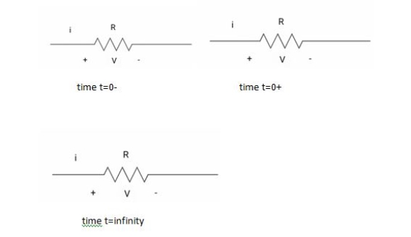
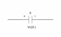
# In case of capacitor: -

At time t= 0-

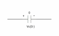
:. Capacitor is initially uncharged

Q (0-) =0

Q=cv

Q (0-) = cvc (0-)

Vc (0-) =0

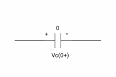
At time t= 0+

By low of conservation of charges

Q (0-) = Q (0+)

Cvc (0-) =cvc (0+)

Vc (0+) =0

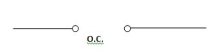
Hence acts as

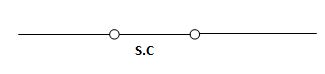
If capacitor is initially uncharged at t= 0- than voltage across capacitor is zero at t=0+ capacitor will follow low of consvation of charges and Vc (0+) =0 it means at t=0+ capacitor behaves as short circuit in other words, voltage across capacitor cannot change instantaneously.

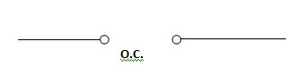
At time t= infinity,

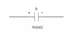
I = cdvc/dt constant and maximum

Hence, i= 0

At t= infinity capacitor will be fully charged or voltage across capacitor is constant and current through capacitor is zero so, capacitor will behave as open –circuit

Say capacitor is initially charged

At time t= 0-,

At time t= 0+,

At time t= 0+

Q (0-) = Q (0+)

Cvc (0-) =cvc (0+)

V1 = Vc (0+)

$C:\Users\TARUNA\AppData\Local\Microsoft\Windows\Temporary Internet Files\Content.Word\IMG_20191229_170304.jpg$

Hence acts as

Its capacitor is initially charged at t= 0- as voltage across capacitor is V1 than at t=0+ capacitor behaves as a voltage as a voltage source with value V1

At time t = infinity

$C:\Users\TARUNA\AppData\Local\Microsoft\Windows\Temporary Internet Files\Content.Word\IMG_20191229_171756.jpg$

If capacitor is initially charged and it is connected to any independent source for long time than current through capacitor is 3 etw and capacitor will be fully charged and it behaves as o.c

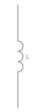
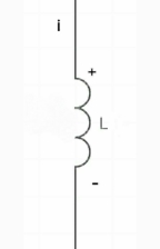
# for Inductor: -

At time t= 0-

$C:\Users\TARUNA\AppData\Local\Microsoft\Windows\Temporary Internet Files\Content.Word\Screenshot_2019-12-29-17-11-12-410_com.miui.gallery.jpg$

Ø= Li =0

Ø (0) = Li (0-)

i (0-) =0

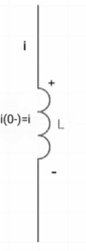
At t= 0+,

$C:\Users\TARUNA\AppData\Local\Microsoft\Windows\Temporary Internet Files\Content.Word\IMG_20191229_172121.jpg$

By low of conservation of flux

Ø (0-) = Ø (0+)

Li (0-) = Li (0+)

0 =i (0+)

Hence, acts as short circuit

System Modelling in terms of Differential Equation:

A linear differential equation which describes any circuit has two parts in its solution, one is complimentary function and other is particular solution. The complimentary solution gives the transient response and the particular solution deals with steady state response. The complete or total response of network is the sum of the transient response and steady state response which is represented by general solution of differential equation.

First order homogenous differential equation.

Integrating both sides

y(t)=k

First order non homogenous differential equation

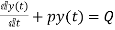
Integrating above equation we get

y(t)=∫ Q

The first term of above solution is known as particular Integral and second is known as complementary function.

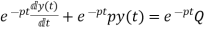
FOR RL Circuit

Fig: Series RL circuit

After switch is closed applying KVL

This is first order homogeneous differential equation so

Integrating both sides

Ln i= t+K

Taking antilog of both sides

i=k

At t=0

i (0) ==I0

=ke0

The particular solution is given as

i= for t≥0

= for t<0

FOR RC Circuit

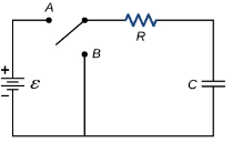
Fig: Series RC circuit

For t>0 applying KVL

Ri(t)++V=0

Hence general solution of above equation is calculated same as for RL circuit

i=k

i (0) =-

Hence, particular solution for network is given as

i=- for t for t≥0

= for t<0

Time Constant

Time constant for RL circuit

From above section for RL circuit at t≥0

i=I0

I0=

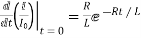
Time taken for current to drop from unity to zero is called as time constant T.

sec

FOR RC Circuit

It can be calculated in the same manner as for series RL circuit

The time constant is given as

T=RC

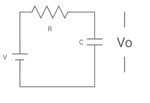
Que: - diagram

$C:\Users\TARUNA\AppData\Local\Microsoft\Windows\Temporary Internet Files\Content.Word\IMG_20191229_221139.jpg$

V0 (t) =? t =o if capacitor is uncharged?

Soln: - diagram

$C:\Users\TARUNA\AppData\Local\Microsoft\Windows\Temporary Internet Files\Content.Word\IMG_20191229_221439.jpg$

Req = R1R2 /R1+R2

V0(0) =0

V0 (infinity) = VR R2/R1+R2

V0 (t) = V0 (infinity) + [Vo (0) – V0 (infinity)] e-t/c

=VR R2/R1+R2 *[ 1- e+(R1+R2)/R1R2]

Ques

Diagram

$C:\Users\TARUNA\AppData\Local\Microsoft\Windows\Temporary Internet Files\Content.Word\IMG_20191229_204756.jpg$

Time constant, c= L/Req = L/R

V(infinity) = 0

V (0) = VR

I(infinity) = VR/R, I (0) =0

By KVL,

VR=i(t) R + L di/dt(t)

On solving

V0(t)= VR e-tR/L

Ques

Diagram

$C:\Users\TARUNA\AppData\Local\Microsoft\Windows\Temporary Internet Files\Content.Word\IMG_20191229_204756.jpg$

Find i(t)

For t>0?

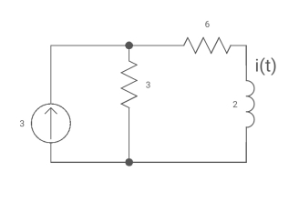
$C:\Users\TARUNA\AppData\Local\Microsoft\Windows\Temporary Internet Files\Content.Word\IMG_20191229_203051.jpg$

Soln

Diagram

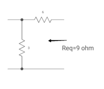
$C:\Users\TARUNA\AppData\Local\Microsoft\Windows\Temporary Internet Files\Content.Word\IMG_20191229_203715.jpg$

Req = 673

= 9 ohms

Diagram

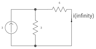
$C:\Users\TARUNA\AppData\Local\Microsoft\Windows\Temporary Internet Files\Content.Word\IMG_20191229_203820.jpg$

T= L/Req = 2/9 sec

I (0) =0

I(infinity) = 3*3/6+3 = 1A

i (+) = 1 [1-e4.51]

Ques

Diagram

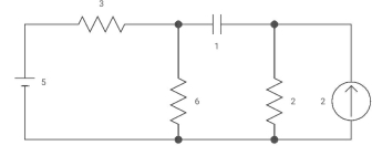
$C:\Users\TARUNA\AppData\Local\Microsoft\Windows\Temporary Internet Files\Content.Word\IMG_20191229_220353.jpg$

Capacitor is initially uncharged find

Vc (t); t >0

Diagram

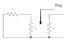
$C:\Users\TARUNA\AppData\Local\Microsoft\Windows\Temporary Internet Files\Content.Word\IMG_20191229_220316.jpg$

Req = (3116) +2

=2+2 = 4ohm

C= c Req

= 2 sec

Clearly Vc (0) =0

Diagram

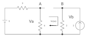
$C:\Users\TARUNA\AppData\Local\Microsoft\Windows\Temporary Internet Files\Content.Word\IMG_20191229_220240.jpg$

By voltage divides, VA = 5*6/3+B = 30 v/9

Clearly by ohms low

VB = 2*2 = 4v

Apply KVL, VA-Vc-VB =0

Vc(infinity) = 30/9 – 4 = -2/3 V

Vc (t) = -2/3 [1- e0.5t]

CURVE: -

Diagram

$C:\Users\TARUNA\Desktop\qq\9.JPG$

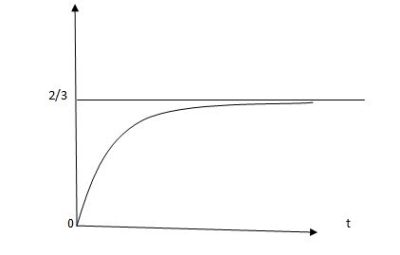
Vc(t) =2/3 [1-e-0.25]

Diagram

$C:\Users\TARUNA\Desktop\qq\544.JPG$

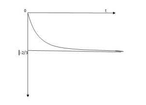
Vc(t) = -2/3 [1-e]

Ques

Diagram

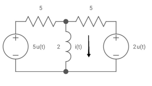
$C:\Users\TARUNA\AppData\Local\Microsoft\Windows\Temporary Internet Files\Content.Word\IMG_20191229_221139.jpg$

(t) =?

Soln: - we know i(t) = I (infinity) + [i (0)- i(infinity0] e-t/c

Diagram

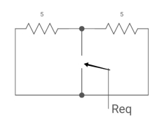
$C:\Users\TARUNA\AppData\Local\Microsoft\Windows\Temporary Internet Files\Content.Word\IMG_20191229_221439.jpg$

Req = 5*5/5+5 = 5?2 ohm

:. T=L/Req = 4/5 sec

Also, i (0) =0

i(infinity) = u(t) +2/5 u(t)

:. I(t) = 1.4 [1-e-5/4t)] u(t)

Transient Response Of R-L, R-C And R-L-C Network in Time Domain

The transient response means the change in the response of output with respect to time. So, using initial conditions, and solution for differential equations we solve some numerical.

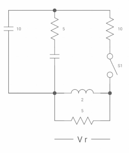
Ques: Diagram

$C:\Users\TARUNA\AppData\Local\Microsoft\Windows\Temporary Internet Files\Content.Word\IMG_20191229_181102.jpg$

If switch ‘s’ closed at t= 0 find out the voltage across capacitor and current through capacitor at t= 0+?

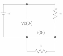
Soln: at t= 0- switch was open so,

$C:\Users\TARUNA\AppData\Local\Microsoft\Windows\Temporary Internet Files\Content.Word\IMG_20191229_175854.jpg$

:. There is no potential so Vc (0-) = 0

At t= 0+, Vc (0-) = Vc (0+) = 0

Diagram

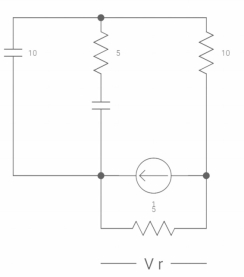
$C:\Users\TARUNA\AppData\Local\Microsoft\Windows\Temporary Internet Files\Content.Word\IMG_20191229_181034.jpg$

Isc = 10/5 = 2 A

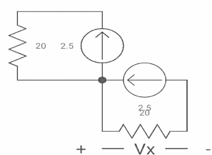
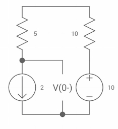
Ques: Diagram

$C:\Users\TARUNA\AppData\Local\Microsoft\Windows\Temporary Internet Files\Content.Word\IMG_20191229_182433.jpg$

The switch was closed for long time before

Opening at t=0- find VX (0+)?

(a) 25V (b) 50 V (c)-50V (d) 0V

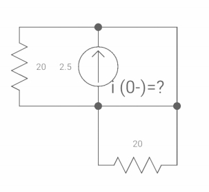
Soln at time t=0-

$C:\Users\TARUNA\Desktop\qq\3.JPG$

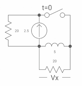
Clearly, il (0-) = 2.5 A

At t= 0+, as inductor is initially charges

So il (0-) = il (0+)

$C:\Users\TARUNA\AppData\Local\Microsoft\Windows\Temporary Internet Files\Content.Word\IMG_20191229_182547.jpg$

-VX= 20/2.5 20*2.5

VX= -50A

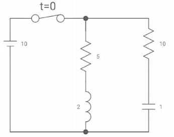
Ques:

$C:\Users\TARUNA\AppData\Local\Microsoft\Windows\Temporary Internet Files\Content.Word\IMG_20191229_183527.jpg$

VR (0+) =

Dil/dt(t) = 0+?

If switch is opened at t= 0?

Soln: -

$C:\Users\TARUNA\AppData\Local\Microsoft\Windows\Temporary Internet Files\Content.Word\IMG_20191229_190915.jpg$

At t=0-

Vc (0-) = 10V

IL (0-) = 10/10 = 1 A

Also, iL (0-) = iL (0+) = 1A

$C:\Users\TARUNA\AppData\Local\Microsoft\Windows\Temporary Internet Files\Content.Word\IMG_20191229_190932.jpg$

VR(0+) = 5V

Ldi(t)/dt = VL (t)

DiL(t)/dt = VL(t)/L

At t= 0+

d/dt iL (0+) = VL (0+)/L

-VL (0+)-VR =0

VL (0+) = -5V

Dt(t) at t = ot = vl (ot)/L

=-5/2

Dil/dt(o+) = 2.5 A/s

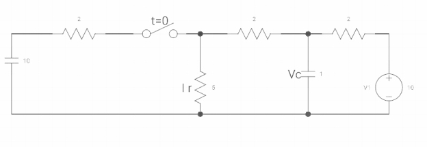
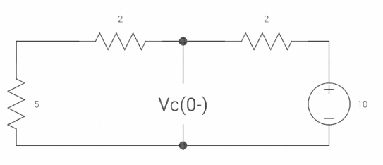
$C:\Users\TARUNA\AppData\Local\Microsoft\Windows\Temporary Internet Files\Content.Word\IMG_20191229_190932.jpg$

Vc(o+) and iR (o+) it switches ‘s’ is closed at t=0?

At t=0

$C:\Users\TARUNA\Desktop\qq\5.JPG$

As capacitor is fully charged so acts as

Vc (0-) = 7*10/7+2 = 70/9v

At t=0+

$C:\Users\TARUNA\AppData\Local\Microsoft\Windows\Temporary Internet Files\Content.Word\IMG_20191229_191007.jpg$

Vc (0+) = Vc (0) = 40/9v

By applying kcl at A,

VA-10/2+ VA/5+VA-7019/2 =0

VA [1/5+1/2+1/2] = 5+35/9

Va [6/5] = 80/9

Va= 400/54v

IR (0+) = Va/5 = 400/54*5 = 80/54 A

2.2 Step, Ramp, sinusoidal and exponential signals by classical method and using Laplace transform

Exponential Rising or Decaying curve

x(t)=x (∞) + [x (0)-x (∞)]

=time constant

From above relation x(t)=0+ [1-0]=

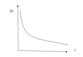
At t= , x (==e-1=0.367

For exponentially decaying signal time at which magnitude of x(t) becomes 36.7% of maximum magnitude of x(t) is called time constant.

x(t)=0+ [1-0]=1-

At t=

x (=0.632.

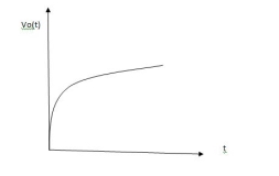
For exponentially rising signal time at which magnitude of x(t) becomes 63.2% of maximum value of x(t) is called time constant.

TRANSIENT RESPONSE :-

Total response = transient response +steady state response

$C:\Users\TARUNA\Desktop\qq\1.png$

V1 –i(t) R-dt=0

Differentiate

0+R+=0

+=0

I.F=

Hence solution is y(t)I. F= IF dx+k

i(t)=k

At t=0, i (0) =k=V1/R

i(t)=

NOTE: Time constant for RC circuit=RC, and for LR circuit =L/R

V0(t)=dt= dt=V1(1- )

The plot for above equations is

$C:\Users\TARUNA\Desktop\qq\7.JPG$ $C:\Users\TARUNA\Desktop\qq\8.JPG$

ALTERNATE METHOD: -

i(t) = i ()+[ i (0)- i ()]

V0(t) =V0 () + [V0(0)-V0()]

And time constant,=C Req

i(0) = V1/ R

i () = 0

V0(0) =0

V0 () = V1

Req = R, =RC

On substituting we get similar results.

Que: -

$C:\Users\TARUNA\AppData\Local\Microsoft\Windows\Temporary Internet Files\Content.Word\IMG_20191229_221139.jpg$

V0 (t) =? t =o if capacitor is uncharged?

Soln: - We know i(t) = i ()+[ i (0)- i ()]

$C:\Users\TARUNA\AppData\Local\Microsoft\Windows\Temporary Internet Files\Content.Word\IMG_20191229_221439.jpg$

Req = R1R2 /R1+R2=(5x5)/ (5+5) =5/2ohm

=L/Req=4/5 sec

i (0) =0

i()=u(t)+u(t)=1.4u(t)

i(t)=1.4[1-]u(t)

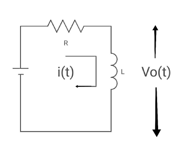
Ques

Diagram

$C:\Users\TARUNA\AppData\Local\Microsoft\Windows\Temporary Internet Files\Content.Word\IMG_20191229_204756.jpg$

Time constant =L/Req = L/R

V () = 0, V (0) =VR (supply voltage)

i () = VR/R, i (0) =0

By KVL,

VR=i(t) R + L di/dt(t)

On solving

V0(t)= VR e-tR/L

Sinusoidal Steady State Analysis:

1) The method used is phasor method.

2) Take Laplace transform of R, L and C in the circuit.

3) Make all initial conditions zero.

4) Derive the expression for desired voltage and current.

5) Replace S by jω where ω is the frequency at which the circuit is operating.

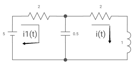
Que) If V1=6cos2t, find i2 at steady state.

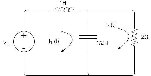
Sol: Apply KVL

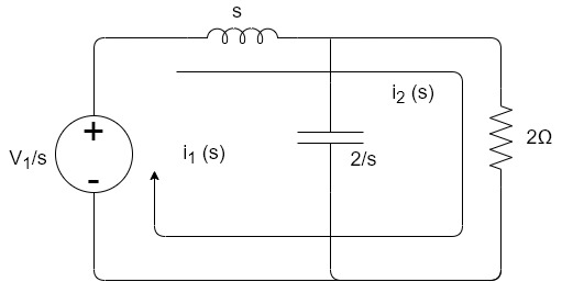
6-sI1(s)-2I2(s)=0

-2I2(s)-I2(s)+ I1(s)=0

I2(s)= I1(s)

I1(s)=[I2(s)

Substituting I1(s) in first equation

6-s[}I2(s)- 2I2(s)=0

Solving above equation we get

I2(s)=

Replace s=jω, s=2j

I2(jω) ===

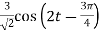
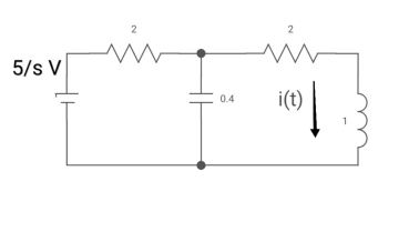
Que) If V1=2sin2t, Va at steady state will be?

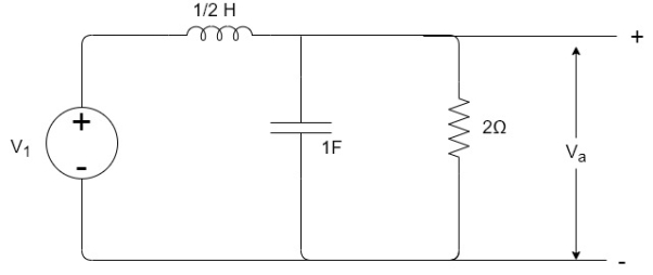
Sol: Zeq=

By voltage divider rule Va=

Replace s by jω , s=2j

Va==

Va=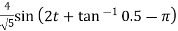

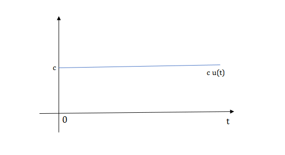
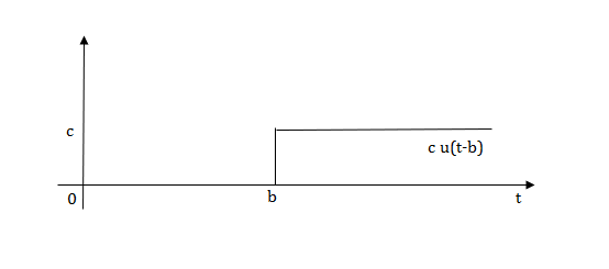
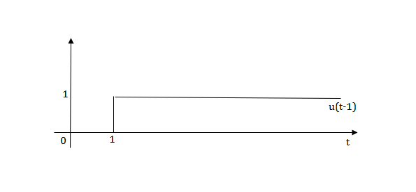
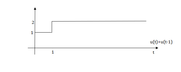
1) Step Function:

U(t)=1 t≥0

=0 t<0

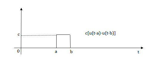
2) Pulse Function:

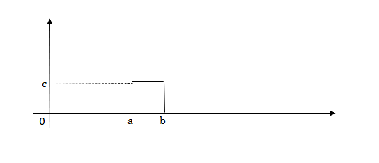
L[u(t)]==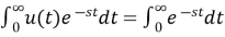

f(t)<—>F(s)

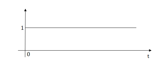
f(t-a)=F(s)

L[u(t-a)]=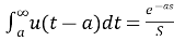

Laplace transforms of pulse

Q.1) Write equation for given waveform

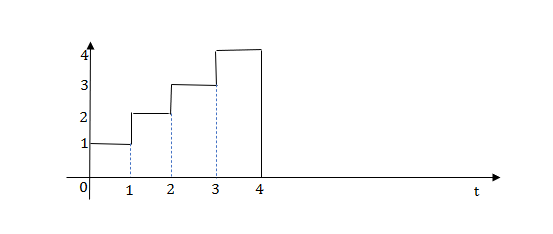
Sol: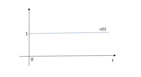

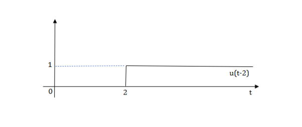
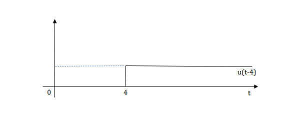
The final equation is=u(t)+u(t-1) +u(t-2) +u(t-3)-4u(t-4)

As the waveform is stopped at t=4 with amplitude 4, so we have to balance that using -4u(t-4).

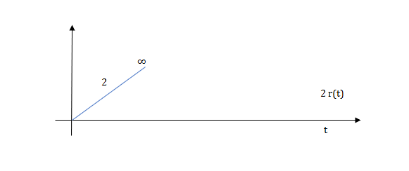
Ramp function:

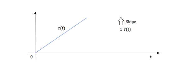
L[r(t)] =

R(t)=tu(t)

R(t)=∫u(t)

Q.3) Write the equation for the given waveform?

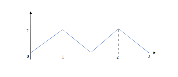
Sol: Calculating slope of above waveform

Slope for (0,0) and (1,2)

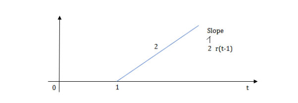
a1 slope==2

a2 slope==-4

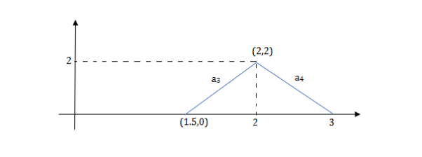
a3 slope =4 and a4= -2

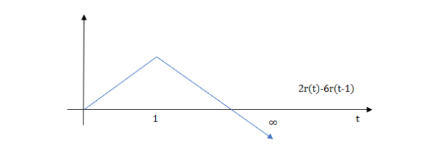
At t=1 slope change from 2 to -4 so we need to add -6r(t-1) to 2r(t) to get the slope of -4.

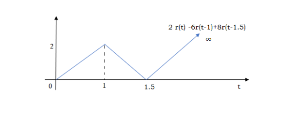
At t=1.5 slope changes from -4 to 4 so adding 8r(t-1.5) to get slope of 4

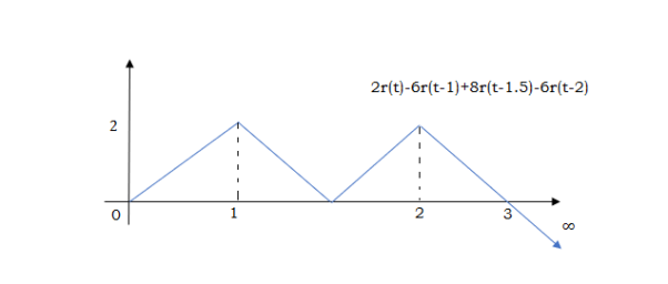
At t=2 slope changes from +4 to -2 so we add -6r(t-2). But we need to stop the waveform at t=3. Hence, we have to make slope 0. Which can be done by adding +2r(t-3). Final equation is given as

2r(t)-6r(t-1.5) +8r(t-1.5)-6r(t-2) +2r(t-3)

Their Laplace transforms, Representation of R, L, C in S domain

If LT[f(t)] = F(s)

Where F(s)=dt

f(t)F(s)

sF(s)-f(0-)

f(t)S2F(s)-sf(0-)-f’(0-)

Now, we find Laplace for

Now if f(t)=ic(t) [current through capacitor]

= [q (0)-q ()]+

=[q(0)-0]+

Multiplying both sides by 1/C

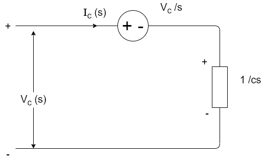
Vc(t)=+

Vc(t)=Vc(0)+

By Laplace Transform

Vc(s)=+

Now by source conversion

Now if f(t)=VL(t) [voltage across inductor]

=-]+

=-0] +

Multiplying both sides by 1/L

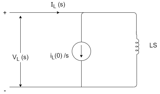
iL(t)=iL(0)+

By Laplace Transform

IL(s)=+

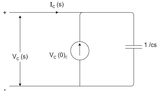
NOTE: Voltage------->Series circuit

Current------->Parallel circuit

By source transformation

Current through capacitor

iC(t)=

IC(s)=C[sVc(s)-Vc(0)]

Vc(s)=+

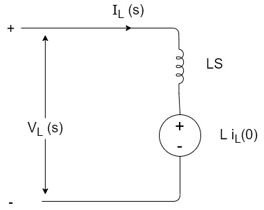
Voltage about inductor,

VL(t)=

VL(s)=L[sIL(s)-iL(0)]

IL(s)=+

Transformed Network

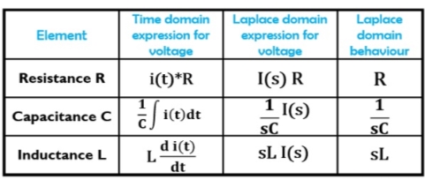
Table for R,L and C and its Laplace Transform

Application of Laplace Transform:

Ques:- Find IL(0)

Diagram

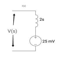
$C:\Users\TARUNA\AppData\Local\Microsoft\Windows\Temporary Internet Files\Content.Word\IMG_20191229_224139.jpg$

Soln: - comparing with ckf,

L = 2H

LiL (0) = 25 mv

IL (0) = 12.5 m A

Que: -

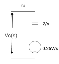
$C:\Users\TARUNA\AppData\Local\Microsoft\Windows\Temporary Internet Files\Content.Word\IMG_20191229_224353.jpg$

Soln: - comparing with circuit,

1/cs = 2/5

C=1/2f

Vc (0)/s = 0.25v/5

Vc (0) = .25v

Ques: -

Diagram

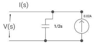
$C:\Users\TARUNA\AppData\Local\Microsoft\Windows\Temporary Internet Files\Content.Word\IMG_20191229_224735.jpg$

Soln: - 1/cs = 1/2S

C=2F

CVc (0) = 0.02

Vc (0) = 0.01

Que: -

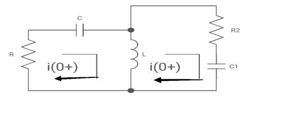
Diagram

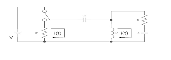
$C:\Users\TARUNA\AppData\Local\Microsoft\Windows\Temporary Internet Files\Content.Word\IMG_20191231_160151.jpg$

(a) switch is at before moving to position = at t= 0, at t= 0+, i1(t) is

(a) –V/2R (b) –V/R (c) – V/4R d0

Soln: -

I1(t) L.T I1(s)

I2(t) L.T I2(s)

Then express in form

[ I1(s)/I2(s)] [:]. [:]

Drawing the ckl at t = 0-

Diagram

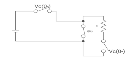
$C:\Users\TARUNA\AppData\Local\Microsoft\Windows\Temporary Internet Files\Content.Word\IMG_20191231_160708.jpg$

:. The capacitor is connected for long

Vc1 = v

IL (0-) = v

IL (0-) =0

Vc2(0-) =0

At t= 0+

Diagram

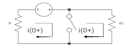
$C:\Users\TARUNA\AppData\Local\Microsoft\Windows\Temporary Internet Files\Content.Word\IMG_20191231_161211.jpg$

$C:\Users\TARUNA\AppData\Local\Microsoft\Windows\Temporary Internet Files\Content.Word\IMG_20191231_161423.jpg$

i1 (0+) = -V/2R

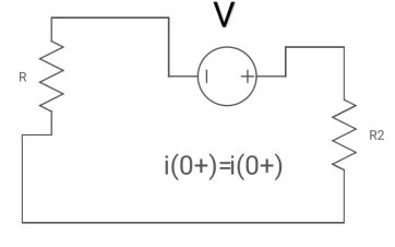
For t>0 he circuits ø

Diagram

$C:\Users\TARUNA\AppData\Local\Microsoft\Windows\Temporary Internet Files\Content.Word\IMG_20191231_161828.jpg$

Apply KVL

-R i1(t) -1/c |i1 (t) dt – Ld./dt [i1(t) - i2 (t)]=0

Also, we can deduce i1(t)- i2 (t) = iL(t)

-RT1(t) -1/c |i1(t)-i2(t) = iL(t)

-RT1(s)- |I1(s)/cs – Vc1(0)/5] – L [ s.I1 (s) – iL (0)]

-RI1(s) –I1(s)/cs –v/s – LS Il(s) =0

-I1(s) [R +1/cs +Ls] – Ls I2(s) = -v/s -------(1)

Again,

-Ri2(t) – 1/c | i2(t) dt – d/dt [i2(t) dt – L d/dt [i2(t)- i1(t)] = 0

-R i2 (t) – 1/c |-1/c |i2(t) dt – L d/dt iL(t) = 0

Taking Laplace transform

- RI2(s) – [I2(s)/cs + vc (00/s] + L [sI1(s)- iL (0) ]= 0

-RI2(s) – I2(s)/cs +Ls [ I1cs) –I2(s)] = 0

I2 (s) [R+1/cs+Ls] – LsT1(s) = 0 --------(2)

Hence, in matrix representation,

[R+1/cs +Ls –Ls [I1(s)] [-v/s]

[-Ls R+1/cs+Ls] [I2 (s)] [0]

Ques: - diagram

$C:\Users\TARUNA\AppData\Local\Microsoft\Windows\Temporary Internet Files\Content.Word\IMG_20191231_162652.jpg$

All initial conditions are zero it L.T, I(s) = ?

Drawing Laplace circuit

$C:\Users\TARUNA\AppData\Local\Microsoft\Windows\Temporary Internet Files\Content.Word\IMG_20191231_162827.jpg$

(2+S) 11 2/S

Zeq = [(2+S)2/S]/[2+S+2/S]=[2(S+2)]/[S2+2s+2]

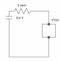
$C:\Users\TARUNA\Desktop\internship\29 dec 2019\IMG_20191228_132621.jpg$

V1(s) = [5/S{2(S+2)/S2+2S+2}]/[2+{2(S+2)/ S2+2S+2}]

V1(s) = [5(S+2)/S]/[S2+ 3S +4]

I(s) = V1(s)/(S+2) = (5/S)/(S2+35+4)

Reference

Engineering Circuit Analysis”, by W H Hayt, TMH Eighth Edition
“Network analysis and synthesis”, by F F Kuo, John Weily and Sons, 2nd Edition.
“Circuit Theory”, by S Salivahanan, Vikas Publishing House 1st Edition, 2014
“Network analysis”, by M. E. Van Valkenburg, PHI, 2000
“Networks and Systems”, by D. R. Choudhary, New Age International, 1999
Electric Circuit”, Bell Oxford Publications, 7th Edition.

Sign Up

Index

Notes

Highlighted

Underlined

Browse by Topics

Notes

Highlighted

Underlined