Unit 5
Content:
- A random variable X is a rule which assigns a number to every outcome e of an experiment. The random variable is a function X(e) that maps the set of experiment outcomes to the set of numbers.
- A random process is a rule that maps every outcome e of an experiment to a function X(t, e).
- A random process is usually conceived of as a function of time, but there is no reason to not consider random processes that are functions of other independent variables, such as spatial coordinates.
- The function X(u, v, e) would be a function whose value depended on the location (u, v) and the outcome e, and could be used in representing random variations in an image.
In the following let’sdeal with one-dimensional random processes to develop a number of basic concepts and then go on to multiple dimensions.
The domain of e is the set of outcomes of the experiment. We assume that a probability distribution is known for this set. The domain of t is a set, T , of real numbers. If T is the real axis then X(t, e) is a continuous-time random process, and if T is the set of integers then X(t, e) is a discrete-time random process
2. We can make the following statements about the random process:
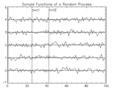
1. It is a family of functions, X(t, e). Imagine a giant strip chart recording in which each pen is identified with a different e. This family of functions is traditionally called an ensemble.
2. A single function X(t, ek) is selected by the outcome ek. This is just a time function that we could call Xk(t). Different outcomes give us different time functions.
3. If t is fixed, say t = t1, then X(t1, e) is a random variable. Its value depends on the outcome e.
4. If both t and e are given then X(t, e) is just a number. The particular interpretation must be understood from the context of the problem
Random processes whose statistics do not depend on time are called stationary. In general, random processes can have joint statistics of any order. If the process is stationary, they are independent of time shift.
The first order statistics are described by the cumulative distribution function F(x;t).
If the process is stationary, then the distribution function at times t = t1 and t = t2 will be identical.
An example of a random process is shown in Figure . At any particular time, F[x;t] = P[X ≤ x;t] is just the cumulative distribution function over the random variable X(t).
The distribution function is independent of time for a stationary process. Given the distribution function, we can compute other first-order statistics such as the probability density.
The second-order statistics are described by the joint statistics of random variables X(t1) and X (t2).
The second-order cumulative distribution function is F(x1, x2;t1, t2)
= P[X(t1) ≤ x1, X(t2) ≤ x2] ------------------------(1)
From which one may compute the density f(x1, x2;t1, t2)
= ∂2F(x1, x2;t1, t2) ∂x1∂x2------------------------ (2)
When the process is stationary these functions depend on the time separation
(t2 − t1) but not on the location of the interval.

The statistics of a random process can be defined for any order n and any set of sample times {t1,...,tn} .
For a stationary process, F [x1,...,xn; xt,...,xt] is independent of translation through time so long as the relative locations of the sample times are maintained.
If the process is stationary for all values of n then it is said to be strict-sense stationary.
Mean
For a discrete random variable X with pdf f(x), the expected value or mean value of X is denoted as E(X) and is calculated as:

For a continuous random variable X with pdf f(x), the expected value or mean value of X is calculated as
E(X) =  . f(x) dx
If the discrete r.v X has a pdf f(x) then the expected value of any function g(X) is computed as
E[g(X)] =  * P(X=x)
Note that E[g(X)] is computed in the same way that E(X) itself is except that g(x) is substituted in place of x.
Covariance
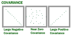
Covariance is a measure of how much two random variables vary together. It’s similar to variance, but where variance tells you how a single variable varies, co variance tells you how two variables vary together.

The Covariance Formula
The formula is:
Cov(X,Y) = Σ E((X-μ)E(Y-ν)) / n-1 where:
X is a random variable
E(X) = μ is the expected value (the mean) of the random variable X and
E(Y) = ν is the expected value (the mean) of the random variable Y
n = the number of items in the data set.
Problem:
Calculate covariance for the following data set:
x: 2.1, 2.5, 3.6, 4.0 (mean = 3.1)
y: 8, 10, 12, 14 (mean = 11)
Substitute the values into the formula and solve:
Cov(X,Y) = ΣE((X-μ)(Y-ν)) / n-1
= (2.1-3.1)(8-11)+(2.5-3.1)(10-11)+(3.6-3.1)(12-11)+(4.0-3.1)(14-11) /(4-1)
= (-1)(-3) + (-0.6)(-1)+(.5)(1)+(0.9)(3) / 3
= 3 + 0.6 + .5 + 2.7 / 3
= 6.8/3
= 2.267
The result is positive, meaning that the variables are positively related.
Consider some function f of time t: f(t)
The average off(t) over finite time interval T is defined and denoted as:
<f(t)>T = 1/T  dt
dt
The average of f(t) over infinite time interval is defined and denoted as
<f(t)>T =lim T->∞ 1/T  dt .
dt .
Definition:
A strict sense stationary process X(t) is said to be strict sense ergodic if all its statistical characteristics can be obtained from ANY of its single realizations x9t) known during an infinite time interval.
Definition 1: A first order stationary process is called 1st order ergodic if any single realization x(t) carries the same information as its 1-dimensional PDD
p1(x,t) = p1(x)
Definition 2: A second order stationary process is called 2nd order ergodic if any single realization x(t) of it carries the same information as its 2-dimensional PDD.
p2(x1,t1,x2,t2) = p2(x1,x2,τ)
Definition 3: An N-th order stationary process is called Nth order ergodic if any single realization x(t) of it carries the same information as its N-dimensional PDD
PN(x1,t1,x2,t2,…………xN,tN) = pN(x1,t1+τ. x2,t2+τ, ………xN,tN,tN+τ)
Consider a 1st order stationary random process X(t), and its particular realization x(t).
If the mean value of the process can be obtained as an average over time of this single realization, i.e.
<x(t)>lim T->∞ 1/T  dt = <x> =
  =
=  p1(x) dx =
The process X(t) is said to be ergodic with respect to mean value.
Definition 4: a 1st order stationary random process X(t) is called ergodic with respect to the mean value, if its mean value can be obtained from any single realization x(t) as the time average of the latter.
Note: • p1 and do not depend on t because the process should be 1st order stationary.
• does not depend on time because it is the result of averaging over time.
Consider a wide sense stationary random process X(t), and its particular realization x(t). Suppose the process is ergodic with respect to mean value. If the covariance of the process can be obtained as an average over time of the product( x(t) -<x>)(x(t+τ) - <x> ),
<(x(t) - <x(t)>) (x(t+τ) - <x(t+τ)>)> = <(x(t) - <x>)(x(t+τ) - <x>)>
= 
Suppose the process is ergodic with respect to mean value. If the covariance of the process can be obtained as an average over time of the product.
Note: • ΨXX(τ) does not depend on t because the process should be wide sense stationary.
• does not depend on time because it is the result of averaging over time. The process X(t) is said to be ergodic with respect to covariance.
Definition 5: a wide sense stationary random process X(t) is called ergodic with respect to covariance, if its covariance can be obtained from any single realization x(t). € (x(t) −x ) (x(t +τ) − x )
Linear Time-Invariant (LTI) Systems:
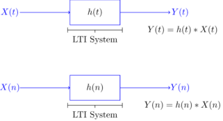
A linear time-invariant (LTI) system can be represented by its impulse response as shown in figure. If X(t) is the input signal to the system, the output, Y(t), can be written as

Y(t) =  X(t-α) dα =
  h(t-α) dα
The above integral is called convolution
Y(t) = h(t) * X(t) = X(t) * h(t)
Note that as the name suggests, the impulse response can be obtained if the input to the system is chosen to be the unit impulse function (delta function) x(t)=δ(t). For discrete-time systems, the output can be written as
Y(n) = h(n) * X(n) = X(n) * h(n)
 X(n-k) =
  h(n-k)
The discrete time unit impulse function is defined as
δ(n) = 1 n=0
0 otherwise
LTI Systems with Random Inputs:
Consider an LTI system with impulse response h(t). Let X(t) be a WSS random process. If X(t) is the input of the system, then the output, Y(t), is also a random process.
More specifically, we can write
Y(t) = h(t) * X(t)
=  X(t-α) dα
Here our goal is to show that X(t) and Y(t) are jointly WSS processes. Let’s first start by calculating the mean function of Y(t) ,μY(t)
We have
μY(t) = E[Y(t)] =E[ X(t-α) dα]
 E[X(t-α)] dα
 E[X(t-α)] dα
 μX(t) dα
= μX(t)  dα
dα
We note that μY(t) is not a function so we can write
μY(t) =μY = μX dα
dα
To find the correlation function RXY(t1,t2) we have
RXY(t1,t2) = E[ X(t1)  X(t2-α) dα ]
= E X1(t) X(t2-α) dα ]
=  E[ X1(t) X(t2-α) ]dα
 Rx(t1,t2-α) dα
 Rx[ t1 -t2 +α) ]dα since X(t) is WSS
We note that RXY(t1,t2) is only a function of  = t1 – t2 so we may write
RXY(τ) =  RX(
RX( +
+  ) dα
) dα
= h(τ) * Rx(-τ) = h(-τ) * RX(τ)
Similarly show that
Ry(τ) = h(τ) * h(-τ) * RX(τ)
From the above results we conclude that X(t) and Y(t) are jointly WSS.
Consider a WSS random process X(t) with autocorrelation function RX(τ). We define the Power Spectral Density (PSD) of X(t) as the Fourier transform of RX(τ). We show the PSD of X(t), by SX(f). More specifically, we can write
SX(f) =  {RX(τ)} =
  e -j2πfτdτ where j= √-1
Power Spectral Density (PSD)
From this definition we conclude that RX(τ) can be obtained by inverse Fourier transform of SX(f)
RX(τ) = F -1 { SX(f)} =  e j2πfτ df
If X(t) is a real-valued random process, then RX(τ) is an even, real-valued function of τ.
From the properties of the Fourier transform, we conclude that SX(f) is also real-valued and an even function of f.
We can conclude that SX(f) is non-negative for all f.
SX(−f)=SX(f), for all f;
SX(f)≥0, for all f.
If we choose τ=0. We know that expected power in X(t) is given by
E[X(t) 2 ] = Rx(0) =  e j2πf0 df=
  df
df
Problem:
Consider a WSS random process X(t) with Rx(τ) = e -a|τ| where a is a positive real number. Find the PSD of X(t)
Solution:
We need to find the Fourier transform of RX(τ).
SX(f) = F{ Rx(τ)}
=  -a|τ| e – j2πfτdτ
=  aτ e – j2πfτdτ +
  -aτ e – j2πfτdτ
= 1/a-j2πf + 1/ a+j2πf
= 2a/ a 2 + 4 π 2 f 2
We describe a Markov chain as follows:
We have a set of states, S = {s1, s2,...,sr}. The process starts in one of these states and moves successively from one state to another. Each move is called a step.
If the chain is currently in state si, then it moves to state sj at the next step with a probability denoted by pij , and this probability does not depend upon which states the chain was in before the current . The probabilities pij are called transition probabilities.
The process can remain in the state it is in, and this occurs with probability pii. An initial probability distribution, defined on S, specifies the starting state. Usually this is done by specifying a particular state as the starting state. R. A. Howard1 provides us with a picturesque description of a Markov chain as a frog jumping on a set of lily pads. The frog starts on one of the pads and then jumps from lily pad to lily pad with the appropriate transition probabilities.
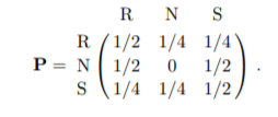
For example According to Kemeny, Snell, and Thompson,2 the Land of Oz is blessed by many things, but not by good weather. They never have two nice days in a row. If they have a nice day, they are just as likely to have snow as rain the next day. If they have snow or rain, they have an even chance of having the same the next day. If there is change from snow or rain, only half of the time is this a change to a nice day.
With this information we form a Markov chain as follows. We take as states the kinds of weather R, N, and S.
From the above information we determine the transition probabilities. These are most conveniently represented in a square array as

Markov Process
A Markov process is a stochastic extension of a finite state automaton. In a Markov process, state transitions are probabilistic, and there is – in contrast to a finite state automaton – no input to the system. Furthermore, the system is only in one state at each time step.
Process diagrams offer a natural way of graphically representing Markov processes – similar to the state diagrams of finite automata.
For example
Cheezit2, a lazy hamster, only knows three places in its cage:
(a) the pine wood shaving that offers him a bedding where it sleeps,
(b) the feeding trough that supplies him with food, and
(c) the wheel where it makes some exercise.
After every minute, the hamster either gets to some other activity, or keeps on doing what he’s just been doing.
Referring to Cheezit as a process without memory is not exaggerated at all:
• When the hamster sleeps, there are 9 chances out of 10 that it won’t wake up the next minute.
• When it wakes up, there is 1 chance out of 2 that it eats and 1 chance out of 2 that it does some exercise.
• The hamster’s meal only lasts for one minute, after which it does something else.
• After eating, there are 3 chances out of 10 that the hamster goes into its wheel, but most notably, there are 7 chances out of 10 that it goes back to sleep.
• Running in the wheel is tiring: there is an 80% chance that the hamster gets tired and goes back to sleep. Otherwise, it keeps running, ignoring fatigue.

Process diagram of a Markov process.
A Markov chain is a sequence of random variables X1, X2, X3, . . . With the Markov property, namely that the probability of any given state Xn only depends on its immediate previous state Xn−1.
P(Xn =x | Xn-1 = xn-1,…………………..X1=x1) = P(Xn=x| Xn-1 = xn-1)
Where P(A | B) is the probability of A given B.
The possible values of Xi form a countable set S called the state space of the chain. If the state space is finite, and the Markov chain time-homogeneous that is the transition probabilities are constant in time, the transition probability distribution can be represented by a matrix P = (pij) i,j , called the transition matrix.
The elements are defined by
Pij = P(Xn =j| Xn-1 =i)
Let x(n) be the probability distribution at time step n, that is a vector whose i-th component describe the probability of the system to be in state i at time state n:
Xi(n) = P(Xn = i)
Transition probabilities can be then computed as power of the transition matrix:
x(n+1) = P · x(n)
x(n+2) = P · x(n+1) = P2 · x(n)
x(n) = Pn·x(0)
References:
An Introduction to Probability and Statistics Book by A. K. Md. Ehsanes Salah and V. K. Rohatgi
Probability and Statistics for Engineering and the Sciences Book by Jay Devore
Probability Theory: The Logic of Science Book by Edwin Thompson Jaynes
Probability and statistics Book by Morris H. DeGroot
Probability, Statistics, and Stochastic Processes Textbook by Peter Olofsson