Unit - 2
Decision Tree Learning
Decision Tree is a Supervised learning technique that can be used for both classification and Regression problems, but mostly it is preferred for solving Classification problems. It is a tree-structured classifier, where internal nodes represent the features of a dataset, branches represent the decision rules and each leaf node represents the outcome.
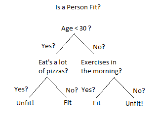
Figure. Decision tree example
In a Decision tree can be divided in to :
- Decision Node
- Leaf Node
Decision nodes are marked by multiple branches that represent different decision conditions whereas output of those decisions is represented by leaf node and do not contain further branches.
The decision test are performed on the basis of features of the given dataset.
It is a graphical representation for getting all the possible solutions to a problem/decision based on given conditions.
Decision Tree algorithm:
- Comes under the family of supervised learning algorithms.
- Unlike other supervised learning algorithms, decision tree algorithm can be used for solving regression and classification problems.
- Are used to create a training model that can use to predict the class or value of the target variable by learning simple decision rules inferred from prior data (training data).
- Can be used for predicting a class label for a record we start from the root of the tree.
- Values of the root attribute are compared with the record’s attribute. On the basis of comparison, branch corresponding to that value is considered and jump to the next node.
2.1.1 Inductive bias
Inductive bias stands for the restrictions that are implied by the assumptions made in the learning method.
Or
An inductive bias of a learner is the set of additional assumptions sufficient to justify its inductive inferences as deductive inferences.
-Tom mitchell
Example:
Assumption: The solution to the problem of road safety can be expressed as a conjunction of a set of eight concepts.it does not allow for more complex expressions that cannot be written as conjunction. Here inductive bias means that there are some potential solutions that we cannot explore, and not contained within the version space that has to be examined.
In order to have an unbiased learner, the version space would have to contain every possible hypothesis that could possibly be expressed.
The solution that the learner produced could never be more general than the complete set of training data.
Similarly it is possible to classify data that learner had previously encountered (as the rote learner could) but would be unable to generalize in order to classify new, unseen data.
The inductive bias of the CEA (candidate elimination algorithm) is that it is only able to classify a new piece of data if all the hypotheses contained within its version space give data the same classification.
Hence, the inductive bias does not impose a limitation on the learning method.
2.1.2 Issues in Decision tree learning
- It is less appropriate for estimation tasks where the goal is to predict the value of a continuous attribute.
- This learning are prone to errors in classification problems with many class and relatively small number of training examples.
- This learning can be computationally expensive to train. The process of growing a decision tree is computationally expensive. At each node, each candidate splitting field must be sorted before its best split can be found. In some algorithms, combinations of fields are used and a search must be made for optimal combining weights. Pruning algorithms can also be expensive since many candidate sub-trees must be formed and compared.
1. Avoiding overfitting
A decision tree’s growth is specified in terms of the number of layers, or depth, it’s allowed to have. The data available to train the decision tree is split into training and testing data and then trees of various sizes are created with the help of the training data and tested on the test data. Cross-validation can also be used as part of this approach. Pruning the tree, on the other hand, involves testing the original tree against pruned versions of it. Leaf nodes are removed from the tree as long as the pruned tree performs better on the test data than the larger tree.
Two approaches to avoid overfitting in decision trees:
- Allow the tree to grow until it overfits and then prune it.
- Prevent the tree from growing too deep by stopping it before it perfectly classifies the training data.
2. Incorporating continuous valued attributes
3. Alternative measures for selecting attributes
- Prone to overfitting.
- Require some kind of measurement as to how well they are doing.
- Need to be careful with parameter tuning.
- Can create biased learned trees if some classes dominate.
KEY TAKEAWAYS
- Decision Tree is a Supervised learning technique that can be used for both classification and Regression problems
- It is a tree-structured classifier, where internal nodes represent the features of a dataset, branches represent the decision rules and each leaf node represents the outcome.
- Two approaches to avoid overfitting in decision trees:
1. Allow the tree to grow until it overfits and then prune it.
2. Prevent the tree from growing too deep by stopping it before it perfectly classifies the training data.
Neural networks are mathematical models that use learning algorithms inspired by the brain to store information. Since neural networks are used in machines, they are collectively called an ‘artificial neural network.’

Nowadays, the term machine learning is often used in this field and is the scientific discipline that is concerned with the design and development of algorithms that allow computers to learn, based on data, such as from sensor data or databases. A major focus of machine-learning research is to automatically learn to recognize complex patterns and make intelligent decisions based on data. Hence, machine learning is closely related to fields such as statistics, data mining, pattern recognition, and artificial intelligence.
Neural networks are a popular framework to perform machine learning, but there are many other machine-learning methods, such as logistic regression, and support vector machines.
Types of Artificial Neural Networks
- FeedForward
- Feedback.
FeedForward ANN
In this ANN:
- Information flow is unidirectional
- A unit sends information to other unit from which it does not receive any information.
- No feedback loops.
- Used in pattern generation/recognition/classification.
- Have fixed inputs and outputs.
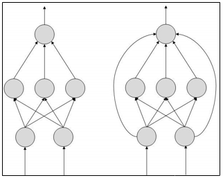
FeedBack ANN
- Feedback loops are allowed.
- Used in content addressable memories.

2.2.1 Perceptrons
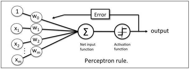
A perceptron is a neural network unit (an artificial neuron) that does certain computations to detect features or business intelligence in the input data.
A Perceptron can also be explained as an algorithm for supervised learning of binary classifiers. It enables neurons to learn and processes elements in the training set one at a time.
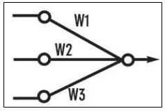
There are two types of Perceptrons:
- Single layer Perceptrons can learn only linearly separable patterns.
- Multilayer Perceptrons or feedforward neural networks with two or more layers have the greater processing power.
The Perceptron algorithm learns the weights for the input signals in order to draw a linear decision boundary.
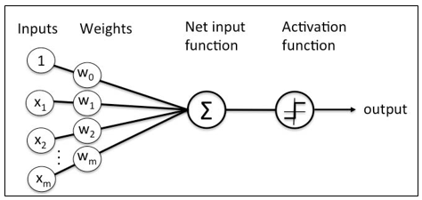
Perceptron Learning Rule
Perceptron Learning Rule states that the algorithm would automatically learn the optimal weight coefficients. The input features are then multiplied with these weights to determine if a neuron fires or not.
The Perceptron receives multiple input signals, and if the sum of the input signals exceeds a certain threshold, it either outputs a signal or does not return an output. In the context of supervised learning and classification, this can then be used to predict the class of a sample.
2.2.2 Gradient descent and the Delta rule
Gradient descent is an optimization algorithm used to find the values of parameters (coefficients) of a function (f) that minimizes a cost function (cost). It is best used when the parameters cannot be calculated analytically (e.g. using linear algebra) and must be searched for by an optimization algorithm.
Types of gradient descent:
• Batch gradient descent refers to calculating the derivative from all training data before calculating an update.
• Stochastic gradient descent refers to calculating the derivative from each training data instance and calculating the update immediately
Generalized Delta Learning Rule
Delta rule works only for the output layer. On the other hand, generalized delta rule, also called as back-propagation rule, is a way of creating the desired values of the hidden layer.
The Delta Rule uses the difference between target activation (i.e., target output values) and obtained activation to drive learning.
Terms used in delta rule:
Threshold activation function & instead a linear sum of products is used to calculate the activation of the output neuron (alternative activation functions can also be applied). That’s why the activation function is called a Linear Activation function, in which the output node’s activation is simply equal to the sum of the network’s respective input/weight products.
The strength of network connections (i.e., the values of the weights) are adjusted to reduce the difference between target and actual output activation (i.e., error).delta rule can be summarized as:
Learning from mistakes.
• “delta”: difference between desired and actual output.
Also called “perceptron learning rule” ∆w = η[y − H wT ( x)]x
2.2.3 Adaline, Multilayer networks
Both Adaline and Perceptron are neural network models of single-layer. Perceptron is oldest and simplest learning algorithms.
Adaline and the Perceptron have similarities:
- Act as classifiers for binary classification
- Both have a linear decision boundary
- Can learn iteratively, sample by sample (the Perceptron naturally, and Adaline via stochastic gradient descent)
- Both use a threshold function
Though Adaline requires continuous predicted values taken from net input to learn the model coefficients, which is more efficient as it can measure the accuracy of our selection.
2.2.4 Derivation of backpropagation rule Backpropagation Algorithm Convergence
The Backpropagation Algorithm is based on generalizing the Widrow-Hoff learning rule. It uses supervised learning, which means that the algorithm is provided with examples of the inputs and outputs that the network should compute, and then the error is calculated.
The backpropagation algorithm starts with random weights, and the goal is to adjust them to reduce this error until the ANN learns the training data.
Standard backpropagation is a gradient descent algorithm in which the network weights are moved along the negative of the gradient of the performance function. The combination of weights that minimizes the error function is considered a solution to the learning problem.
The backpropagation algorithm requires a differentiable activation function, and the most commonly used are tan-sigmoid, log-sigmoid, and, occasionally, linear. Feed-forward networks often have one or more hidden layers of sigmoid neurons followed by an output layer of linear neurons. This structure allows the network to learn nonlinear and linear relationships between input and output vectors. The linear output layer lets the network get values outside the range − 1 to + 1.
For the learning process, the data must be divided in two sets:
- Training data set, which is used to calculate the error gradients and to update the weights;
- Validation data set, which allows selecting the optimum number of iterations to avoid overlearning.
As the number of iterations increases, the training error reduces whereas the validation data set error begins to drop, then reaches a minimum and finally increases. Continuing the learning process after the validation error arrives at a minimum leads to overlearning. Once the learning process is finished, another data set (test set) is used to validate and confirm the prediction accuracy.
Properly trained backpropagation networks tend to give reasonable answers when presented with new inputs.Usually, in ANN approaches, data normalization is necessary before starting the training process to ensure that the influence of the input variable in the course of model building is not biased by the magnitude of its native values, or its range of variation. The normalization technique, usually consists of a linear transformation of the input/output variables to the range (0, 1).
Feedforward Dynamics
When a BackPropagation network is cycled, the activations of the input units are propagated forward to the output layer through the connecting weights. As in perceptron, the net input to a unit is determined by the weighted sum of its inputs:
Netj = iwjiai
Where ai is the input activation from unit i and wji is the weight connecting unit i to unit j. However, instead of calculating a binary output, the net input is added to the unit's bias and the resulting value is passed through a sigmoid function:
F(netj) = 1/(1 + e-netj+ j ).
The bias term plays the same role as the threshold in the perceptron. But unlike binary output of the perceptron, the output of a sigmoid is a continuous real-value between 0 and 1. The sigmoid function is sometimes called a "squashing" function because it maps its inputs onto a fixed range.
2.2.5 Generalization
Generalization refers to the model’s ability to respond to a new set of data.after being trained on a training set, a model can ingest new data and initiate making accurate predictions.
A model’s ability to generalize is vital to the success of a model. If a model has been trained too well on training data, it will be unable to generalize. It will make inaccurate predictions when provided with new data, making the model useless even though it is able to make accurate predictions for the training data. This process is called overfitting. The inverse is Underfitting that happens when a model has not been trained enough on the data. In case of underfitting, even with the training data, model is found incapable of making accurate predictions,
Figure demonstrates the three concepts given above.

On the left, the blue line represents a model that is underfitting.
The model notes that there is some trend in the data, but it is not specific enough to capture relevant
It is unable to make accurate predictions for training or new data. In the middle,
The blue line represents a model that is balanced. This model notes there is a trend in the data, and accurately models it.
This middle model will be able to generalize successfully. On the right, the blue line represents a model that is overfitting.
The model notes a trend in the data, and accurately models the training data, but it is too specific. It will fail to make accurate predictions with new data because it learned the training data too well.
KEY TAKEAWAYS
- Neural networks are a popular framework to perform machine learning, but there are many other machine-learning methods, such as logistic regression, and support vector machines.
- Types of Artificial Neural Networks: Feed Forward , Feedback
- The Delta Rule uses the difference between target activation (i.e., target output values) and obtained activation to drive learning.
- The Backpropagation Algorithm is based on generalizing the
Widrow-Hoff learning rule.
References:
1. Tom M. Mitchell, ―Machine Learning, McGraw-Hill Education (India) Private Limited, 2013.
2. Ethem Alpaydin, ―Introduction to Machine Learning (Adaptive Computation And Machine Learning), The MIT Press 2004.
3. Stephen Marsland, ―Machine Learning: An Algorithmic Perspective, CRC Press, 2009.
4. Bishop, C., Pattern Recognition, and Machine Learning. Berlin: Springer-Verlag.