Consider a temperature control system for a room as shown in figure 1. If temperature of thermostat is increased from 20 to 25
to 25 . As input to control system changes so output will also change. We need mathematical model in order to determine the how output of control system will react to different inputs i.e. we need equations describing how the input and output of control system are related to each other. Using these equations, we can predict how output will react to input changes. We are also concern with how output will respond with time as changes to required value.
|
Figure 1: Temperature control system for a room.
Static response:
Static response is defined as response of system to input without consideration of time taken to reach that response. For example consider an amplifier system as show in figure 2. If we have an input of magnitude 2 V then output will be 20 V. This is a simple system model where the input is multiplied by a gain of 10 in order to give the output and we are looking at just the static response.
|
Figure 2: Amplifier system with the output 10 times the input.
Dynamic response:
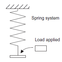
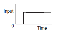
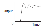
Dynamic response is defined as response of system to input with consideration of time taken to reach that response. Consider a simple spring balance system where load is input and output of system will deflection of spring as shown in figure 3A. Applied load to system is acts as step input because input variation with time looks like step as shown in figure 3B. As we know spring balance system will not instantaneously give the weight but the pointer on the spring balance will oscillate for a little time before spring balance the applied the load value. Weight value is static response to which spring balance eventually settles down to. But, for a complete behaviour of the spring balance system with time, we cannot consider for an input of some constant load, that the output is just the input multiplied by some constant number but need some way of describing mathematical model by which an output varies with time.
|
Figure 3: Spring balance system
A: The spring system with constant load B: the step showing how the C: The output showing is applied at some instant of time input varies with time how it varies with time for the step input.
Gain
Consider a system where output is direct proportional to input mathematically
Where G is constant known as gain. |
Gain of system in series
Consider two system e.g., amplifier are arranged in series with having gain For first system
Also for second system
We can say that for overall system Thus we can say
Where For series-connected systems, the overall gain is the product of the gains of the constituent systems. |
Feedback loops
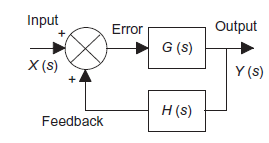
Consider a system model with negative feedback loop. Output of system is fed back via measurement system with gain H to subtract from input X to system with gain G.
Input to feedback system is y hence output is yH. And error is X-Hy
Y=G(X-Hy)
Overall gain of system =Y/X=G/(1+GH) |
Path from the error signal to the output is known as forward path and so, in this case, the forward path gain is G. Path from the output back to the comparison element is known as feedback path and so, in this case, the feedback path gain is H. Thus, for a system with a negative feedback, the overall gain is the forward path gain divided by one plus the product of the forward path and feedback path gains.
Similarly, for positive feedback path
Overall gain of system=G/(1-GH)
Dynamic system
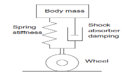
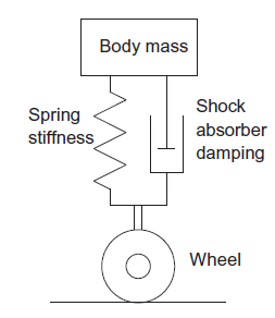
We need mathematical model to describe relationship between input and output of system as well as how output will varies with respect to time. To describe relationship between input and output we can consider a whole system constitute of simple basic elements. For example consider an automobile suspension system how it extend or compress it, i.e. its stiffness, the forces damping out any motion of the suspension and the mass of the system and so its resistance of the system to acceleration, i.e. its inertia. So we think of the model as having the separate elements of stiffness, damping and inertia which we can represent by a spring, a dashpot and a mass as shown in figure 4 and then write down equations for the behaviour of each element using the fundamental physical laws governing the behaviour of each element. This way of modelling a system is known as lumped-parameter modelling.
|
Figure 4: An automobile suspension system
Mechanical system
Mechanical systems have stiffness, damping and inertia and can be considered to be composed of basic elements which can be represented by springs, dashpots and masses as shown in figure 5.
Spring
Stiffness of spring can be represented by ideal spring as shown in figure 5A. For linear spring extension (y) is directly proportional to applied force (F). Mathematically
F=k*y
Where k = stiffness of spring
Dashpot
Damping of mechanical system can be represented as dashpot as shown in figure 5B. This is piston moving in viscous medium. When piston moves inwards the trapped fluid flows out past edges of the piston and when piston moves outwards fluids flow past the piston and into the enclosed space. For such a system, the resistive force F has to be overcome is proportional to the velocity of the piston and hence the rate of change of displacement y with time, i.e., dy/dt. Mathematically

Where c = damping constant
Mass
Inertia of system is means resistance of system when it is accelerated can be represented as mass. As shown in figure 5C by Newton’s second law F = ma. But acceleration is change in velocity v with time and velocity is change in displacement y with time. Mathematically

|
A: Spring B: Dashpot C: Mass
Figure 5: Basic mechanical element
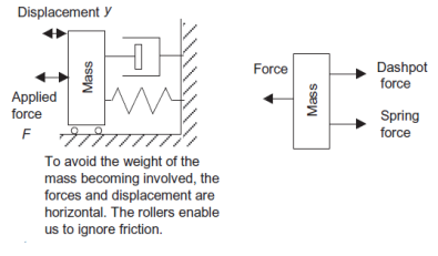
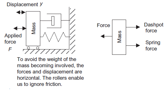
Consider a mechanical system consists of spring, dashpot and mass as shown in figure 6. Input to system is force (F) and output is displacement (y).
|
Figure 6: Mechanical system with mass, damping and stiffness
From free body diagram (from figure 6) Net force = F - ky - By newton’s second law
net force =
|
Rotational system
In control systems we are often concerned with rotational systems e.g. model for the behaviour of a motor drive shaft. How the driven load rotation will be related to the rotational twisting input to the drive shaft. Basic building blocks for rotational system are a torsion spring, a rotary damper and the moment of inertia as shown in figure 7
|
Figure 7: Basic rotational elements
Torsional spring
For a torsional spring, the angle θ rotated is proportional to the torque T, mathematically
T= k
Where
k=stiffness of spring
Rotational dashpot
For a rotational dashpot, the resistive torque T is proportional to the angular velocity ω and thus
T = cω = c
Where c = damping constant.
Inertia
The inertia of a rotational system is represented by the moment of inertia of a mass. A torque T applied to a mass with a moment of inertia I results in an angular acceleration .
.
T= I  =I
=I
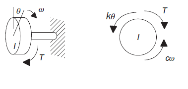
Consider a rotational system as shown in figure 8 rotation disk as a result of twisting a shaft.
|
Figure 8: Rotational system with FBD
The torques acting on the disk are the applied torque T, the spring torque kθ and the damping torque cω. T – k
|
Electrical system
The basic elements of electrical systems are the pure components of resistor, inductor and capacitor i.e. resistor only possesses the property of resistance, the inductor possesses the property of inductance and the capacitor possesses the property of capacitance as shown in figure 9.
|
Figure 9: Basic electrical element
Resistor
For a resistor, resistance R is the potential difference v across it when there is a current i through it. Mathematically
v=iR
Inductor
For an inductor, inductance L, the potential difference v across it at any instant depends on the rate of change of current i. mathematically
V=L
Capacitance
For a capacitor, the potential difference v across it depends on the charge q on the capacitor plates with v=q/C, where C is the capacitance. Mathematically
v = 

But i = 

The relationship between the output and input is given by a differential equation when input and output are function of time. For complex system it is difficult to obtain input-output relationship in differential equation form. So we need to transform these differential forms into more convenient and easy form using Laplace transform so we can easily manipulate by basic rule of algebra.
For transformation we follow following rules:
i.e.
i.e.
Note that, when derivatives are involved, we need to know the initial conditions of a system output prior to the input being applied before we can transform a time function into an s function.
|
We know gain G= output/input.
When input and output are the function of s
Transfer function G(s)=Y(s)/X(s) when all initial conditions are zero before we apply input.
Transfer function can be represented as block diagram as shown in figure below
|
Figure 10: Transfer function as the factor that multiplies the input to give the output
Where,
X(s )=input function of s
Y(s)= output function of s
G(s)= transfer function as the operator in the box that converts the input to the output.
Transfer function of common system elements
Transfer function for system can obtain by considering relationship between input to system and their output. We can describe any control system as series of interconnected blocks and each block have its input-output characteristics defined by a transfer function. Following table is for transfer functions which are commonly encounter system elements.
Control system |
|
Gear train | For the relationship between the input speed and output speed with a gear train having a gear ratio N: Transfer function = N |
Amplifier | For the relationship between the output voltage and the input voltage with G as the constant gain Transfer function = G |
Potentiometer | For the potentiometer acting as a simple potential divider circuit the relationship between the output voltage and the input voltage is the ratio of the resistance across which the output is tapped to the total resistance across which the supply voltage is applied and so is a constant and hence the transfer function is a constant K: Transfer function=K |
Armature-controlled DC motor | For the relationship between the drive shaft speed and the input voltage to the armature is Transfer function
where L =inductance of the armature circuit and R =resistance |
Valve controlled hydraulic actuator | The output displacement of the hydraulic cylinder is related to the input displacement of the valve shaft by a transfer function of the form Transfer function = where K1, K2 and K3 are constants |
Heating system | The relationship between the resulting temperature and the input to a heating element is typically of the form: Transfer function= where C = thermal capacity of the system and R = thermal resistance |
Tachogenerator | The relationship between the output voltage and the input rotational speed is likely to be a constant K and so represented by Transfer function = K |
Displacement and rotation | For a system where the input is the rotation of a shaft and the output, as perhaps the result of the rotation of a screw, a displacement, since speed is the rate of displacement we have v= dy/dt and so V(s)=sY(s) and the transfer function = 1/s
|
Height of liquid level in a container | The height of liquid in a container depends on the rate at which liquid enters the container and the rate at which it is leaving. The relationship between the input of the rate of liquid entering and the height of liquid in the container is of the form Transfer function = Where A = cross-sectional area of the container, ρ = density of the liquid, g = acceleration due to gravity and R = hydraulic resistance offered by the pipe through which the liquid leaves the container. |
Transfer function and systems
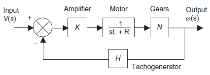
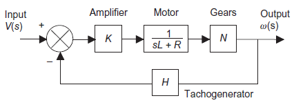
Consider speed control system consisting of differential amplifier, drive motor, gear system, driving shaft and tachogenerator.

|
Figure 11: Block diagram for the control system for speed of a shaft
Note: Terms in the boxes are the transfer functions for the elements concerned.
System transfer functions
Overall transfer function of any control system consists of series of connected elements and system with feedback loops.
Systems in series
Consider a system consisting of two subsystems in series as shown in figure 12.
|
Figure 12: Systems in series
From figure 12 X(s) is input to first subsystem and output is 
Transfer function of first subsystem is
Second subsystem has Transfer function of second subsystem is
Overall transfer function for system is
|
Thus, we can say that overall transfer function of system is product of transfer function of individual series elements.
Systems with feedback
System with negative feedback.
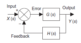
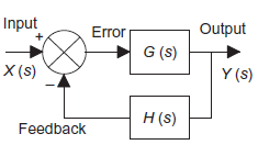
Consider a system with negative feedback loop as shown in figure 13. Where the output Y(s)is fed back via a system with a transfer function H(s) to subtract from the input X(s) to the system having G(s) as transfer function
|
Figure 13: System with negative feedback.
Input for feedback system is Y(s) and output is H(s)Y(s).
The error is the difference between the system input signal X(s) and the feedback signal H(s)Y(s)
Error= X(s)-H(s)Y(s)
This error is input to system G(s) and output is Y(s)
|
System with positive feedback
|
Figure 14: System with positive feedback
Error= X(s)+H(s)Y(s) This error is input to system G(s) and output is Y(s)
|
Block manipulation
Complex systems have many elements and sometimes more than one input. Following are some ways to reorganise the blocks in simplified way and still give the same overall transfer function for given system.
| System | Equivalent system |
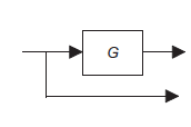
Blocks in series |
|
|
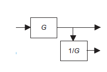
Moving a take-off point to beyond a block |
|
|
Moving a take-off point to ahead of a block |
|
|
Rearrangement of summing points |
|
|
Interchange of summing points. |
|
|
Moving a summing point ahead of a block. |
|
|
Moving a summing point beyond a block |
|
|
Removing a block from a feedback path |
|
|
Removing a block from a forward path. |
|
|
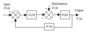
Multiple inputs
When systems have more than one input superposition principle can be used.
Superposition principle: The response to several inputs simultaneously applied is the sum of the individual responses to each input when applied separately.
Following described procedure is for multiple inputs - single output (MISO) system
Sensitivity
Sensitivity of control system is defined as how much the output varying with respective to variation of system parameters. As transfer function may drift with time and it is necessary to find out how this drift will affect the performance of control system.
Consider a closed loop system with negative feedback as shown in figure 15.
|
Figure 15: System with negative feedback.
If Overall transfer function
|
From above equation we can say that system is relatively insensitive to forward path function but sensitive to variations in feedback path transfer function. For example, a change in the feedback path transfer function of, say, 10%, i.e., from H(s) to 1.1H(s), will result in a change in the overall transfer function from 1/H(s) to 1/1.1H(s) or about 0.9/H(s) and so a change of about 10%. The reason for this sensitivity is because the feedback transfer function is for the measurement system supplying the signal which is compared with the set value signal to determine the error and so variations in the feedback transfer function directly affect the computation of the error.
If forward path function G(s) changes then overall transfer function  will also change. So sensitivity for control system can be defined as ratio of changes in the transfer function of the forward element as the fractional change in the overall system transfer function
  divided by the fractional change in the forward element transfer function G(s). Mathematically
Differentiate the equation given above for the overall transfer function we obtain
Since
|
From above equation we can say that sensitivity is minimum if  is maximum.
Sensitivity to Disturbances
Reduction in disturbance signal is most important effect of having feedback in system. Disturbance signal is nothing but unwanted signal which affects the output of system, e.g. continuous opening and closing of door of air conditioned room.
Consider an open loop system as shown in figure 16.
|
Figure 16: Disturbance with an open-loop system
Overall system output is given as
|
Now consider a closed loop system as shown in figure 17
|
Figure 17: Disturbance with closed-loop system.
Overall system output is given as
|
If we compare overall output of both systems, we can conclude that the effect of the disturbance on the output of the system has been reduced by a factor of  this factor is thus a measure of how much the effects of a disturbance are reduced by feedback.
System response
Inputs
Step input: Input suddenly being switched to a constant value at some particular time. Figure 18A
Impulse input: Input existing for just a very brief time before dropping back to zero. Figure 18B
Ramp input: Input existing for just a very brief time before dropping back to zero. Figure 18C
|
Figure 18: Forms of input
Determining outputs
The procedure for determining how the output of a system will change with time when there is some input to the system is:
In terms of transfer function G(s)
Output(s)=G(s)*Input(s)
i.e. output of system as a Laplace transform by multiplying its transfer function by Laplace transform of input.
2. Determine the time function corresponding to the output transform.
To determing output as a function of time find the time function that will give the particular
output transform that we have obtained i.e. find inverse transform.
|
Partial fraction
Partial fraction is techniqe used to find inverse transformation. Partial fraction helps to convert complex fraction into simpler fraction terms. There are basically three types of partial fractions:


Expression form | Partial fraction |
|
|
|
|
|
|
First order system Differential equation for first order system is given as
Where T= time constant K= steady state gain Generally first order system have capacitive and resistive element for example a temperature sensor is typically a first-order system. Laplace transform of above equation is gives as
Transfer function When a first-order system is subject to a unit impulse input then
Taking laplace inverse
When a first-order system is subject to a unit step input then X(s)=1/s and output transform Y(s) is
Taking Laplace inverse, we get y= k(1- First-Order System Parameters
When t=T T= time constant Then we have Thus, the time constant T for a first-order system when subject to a step input is the time taken for the output to reach 0.63 of the steady-state value
Time required for the output response to reach 50% of its steady-state value is known as delay time Thus, since k is the final value, the time taken to reach 50% of this value is given by
Time required for the output to rise from 10% to 90% of its steady-state value is known as rise time Since k is the steady-state value then the time taken to reach 10% of that value is
Similarly The time taken to reach 90% of the steady-state value is given by
Rise in time
Second order systems Idling control system used with a car engine is an example of a control system which behaves as a second-order system. is the. When there is a sudden change in engine load the engine speed must not drop and cause the engine to stall, thus any transient drop must not be excessive and the speed should recover to the required idling speed as fast as possible. The differential equation for a second-order system is of the form
Where
Taking Laplace transform
Transfer function When a second-order system is subject to a unit step input i.e. X(s)=1/s
There are three different forms of answer to this equation for the way the output varies with time; these depending on the value of the damping constant and whether it gives an over-damped, critically damped or under-damped system. We can determine the condition for these three forms of output by putting the equation in the form
where
For this condition roots are real and will factorise Taking Laplace inverse transform
This describes an output which does not oscillate but dies away with time and thus the system is overdamped. As the time t tends to infinity then the exponential terms tend to zero and the output becomes the steady value of
square root terms becomes zero
This equation can be expanded by means of partial fractions to give
Hence:
This is the critically damped condition and describes an output which does not oscillate but dies away with time. As the time t tends to infinity then the exponential terms tend to zero and the output tends to the steady-state value of k.
With ζ =1 the square root term does not have a real value
Where cos This is an under-damped oscillation. The angular frequency of the damped oscillation is
Only when the damping is very small does the angular frequency of the oscillation become nearly the natural angular frequency
Second order system parameter For the under-damped oscillations of a system we have the output y given by
with the damped frequency ω given by
and since φ is a constant
where P and Q are constants. Thus the output can be written as
|
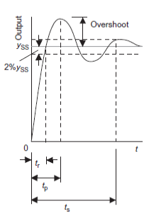
The performance of an under-damped second-order system to a unit step input (Figure 19) can be specified by:
|
Figure 19: Step response of an under-damped system
time taken for the response x to rise from 0 to the steady-state value This is the time for the oscillating response to complete a quarter of a cycle
To reduce the rise time by increasing the damped natural frequency, this value being determined by the undamped natural angular frequency and the damping factor.
Sometimes rise time can specified as the time taken for the response to rise from 10% to 90% of the steady-state value.
Time taken for the response to rise from 0 to the first peak value is known as peak time. This is the time for the oscillating response to complete one half-cycle
When ζ is 1 then the peak time becomes infinite; this indicates that at critical damping the steady-state value is never reached but only approached asymptotically.
Maximum amount by which the response overshoots the steady-state value is known as overshoot. and is thus the amplitude of the first peak. The overshoot is often written as a percentage of the steady-state value. The steady-state value is when t tends to infinity and thus then using:
The overshoot occurs at ωt=π and thus
The overshoot is the difference between the output at that time and the steady-state value. Hence
We know
Therefore Expressed as a percentage of
An indication of how fast oscillations decay is provided by the subsidence ratio or decrement. This is the amplitude of the second overshoot divided by the amplitude of the first overshoot. The first overshoot occurs when we have ωt=π and so
The second overshoot occurs when ωt=3π
Thus the subsidence ratio is given by
Time taken for the oscillations to die away is known as settling time
The time taken to complete one cycle, is 1/f, where f is the frequency, and since ω=2πf then the time to complete one cycle is 2π/f. In a settling time of ts the number of oscillations that occur is
and thus for a settling time defined for 2% of the steady-state value Number of oscillations = We know
Number of oscillations =
|
Sinusoidal signals
If input is sinusoidal signal then steady state output will also be sinusoidal with same frequency but sometimes magnitude or amplitude and phase  can be differ between in input and output (figure 19). Sinusoidal signals are represented by phasors. Consider a sinusoidal signal
Where,
Y= amplitude,  =angular frequency
Sinusoidal inputs
For step and impulse inputs we are interested in transient and steady state responses but for sinusoidal inputs we are only interested in steady state response. Frequency response of system means steady state response of the system to a sinusoidal input signal. The steady state output is a sinusoidal signal of the same frequency as the input signal, differing only in amplitude and phase angle.
The frequency response of a system can be found by applying a sinusoidal input signal to the input of the system and measuring the output so that the gain and the phase can be determined. Such measurements can be carried out for a number of frequencies.
Frequency response function
The procedure for determining the frequency response of a system is as follows:


Frequency response for a first-order system
First order transfer can be written as
Where
|
The frequency response function
Multiplying denominator and numerator by We get
This is of the form
The phase difference f between the output phasor and the input phasor is given by
The negative sign indicates that the output phasor lags behind the input phasor by this angle. Frequency response for a second-order system Consider a second-order system with the transfer function
Where,
The frequency response function
On simplifying we get
Multiplying denominator and numerator by We get
This is of the form
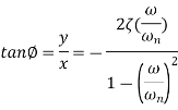
The phase difference f between the output phasor and the input phasor is given by
The negative sign indicates that the output phasor lags behind the input phasor by this angle.
|
Bode plot
As frequency response of system is set values of magnitude  and phase angle
  . This can expressed as two graphs one is magnitude
  against angular frequency
  and other one is phase
  against angular frequency
 . Magnitude and angular frequency are plotted using logarithmic scales. These pair of graph is referred as bode plot.
Magnitude is expressed is in decibel units (dB)
Bode plot for G(s) = K Consider a system with Transfer function G(s) = K Where K= constant. Frequency response function for system is Magnitude Magnitude plot is thus a line of constant magnitude thus changing K shifts magnitude line up and down and the phase is zero. Figure 20 shows Bode plot for G(s)=K |
|
Figure 20: Bode plot for G(s)=K
Bode plot for G(s) = 1/s
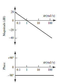
Consider a system with Transfer function G(s) = 1/s Frequency response function for system is Multiplying denominator and numerator by
|
|
Figure 21: Bode plot for G(s)=1/s
In decibels When When When Phase of system is given as Figure 21 shows bode plot for G(s)=1/s
|
Bode plot for a first-order system
Frequency response for a first-order system
First order transfer can be written as
Where
The frequency response function
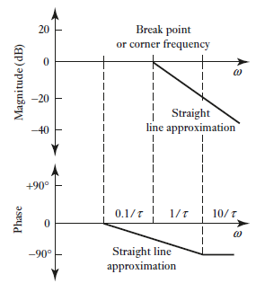
Magnitude In decibels If Hence at low frequencies there is a straight line magnitude plot at a constant value of 0 dB. If Magnitude is 20log( This is a straight line of slope -20 dB per decade of frequency which intersects the 0 dB line when , The phase for the first-order system is given by
the phase is virtually 0°at low frequency when Figure 22 shows Bode plot for first order system.
|
|
Figure 22: Bode plot for first order system
Bode plot for a second-order system
Consider a second-order system with the transfer function
Where,
The frequency response function
In decibels magnitude is For For The magnitude plot is thus approximately given by these two asymptotic lines. The true value, however, depends on the damping ratio Phase is given by For For When |
|
Figure 23: Bode plot for a second-order system.
Building up Bode plot
Consider system with number of elements in series with transfer function given as
Frequency response can be obtain by replacing s by
We can write the transfer function
Where Similarly, for
On simplifying
The frequency-response function of the system has a magnitude, which is the product of the magnitudes of the separate elements, and a phase, which is the sum of the phases of the separate elements, i.e.
Now, considering the Bode plot where the logarithms of the magnitudes are plotted,
|
Thus, we can obtain the Bode plot of a system by adding together the Bode plots of the magnitudes of the constituent elements. Likewise, the phase plot is obtained by adding together the phases of the constituent elements.
Nyquist diagram is method is used for describing frequency response of system and their stability. In these diagrams gain and phase of open loop transfer function are plotted are as polar graphs for various values of frequency. In polar graph points are plotted from the origin according to their radial distance from it and their angle to reference axis as shown in figure 24. The Nyquist diagram is the line joining the series of points plotted on a polar graph when each point represents the magnitude and phase of the open-loop frequency response corresponding to a particular frequency. To plot the Nyquist diagram from the open-loop transfer function of a system we need to determine the magnitude and the phase as functions of frequency.
|
Figure 24: Polar graph with points specified by r and  values
Polar plot
Polar plot of the frequency response of a system traced out as the frequency is changed from 0 to infinity by the tips of the phasors whose lengths represent the magnitude, i.e. amplitude gain, of the system and which are drawn at angles corresponding to their phase as shown in figure 25
.
|
Figure 25: Polar plot with the plot as the line traced out by the tips of the phasors as the frequency is changed from zero to infinity
Nyquist stability criteria
Closed-loop systems whose open-loop frequency response G(jω)H(jω) as ω goes from 0 to infinity does not encircle the -1 point will be stable, those which encircle the -1 point are unstable and those which pass through the -1 point are marginally stable. Encircling the point may be taken as passing to the left of the point. Figure 26 Explains above with examples of stable, marginally stable, and unstable systems. The Nyquist plots, not to scale, correspond to the open-loop frequency response of:
|
|
Figure 26: Stability and the Nyquist plot.
with K=10 for the stable plot, K=137 for the marginally stable plot and K=500 for the unstable plot. The vertical axis of the Nyquist plot corresponds to the phase equal to 90 and so is the imaginary part of the open-loop frequency response. The horizontal axis corresponds to the phase equal to 0
 and so is the real part of the open-loop frequency response.
References:
1. Instrumentation and control systems by W. Bolton, 2nd edition, Newnes, 2000.
2. Thomas G. Beckwith, Roy D. Marangoni, John H. Lienhard V, Mechanical Measurements (6th Edition) 6th Edition, Pearson Education India, 2007.
3. Gregory K. McMillan, Process/Industrial Instruments and Controls Handbook, Fifth Edition, McGraw-Hill: New York, 1999.


