UNIT 3

Pricing under imperfect market condition

3.1 Meaning of Imperfect Competition

Imperfect competition is a competitive market where a large number of sellers are engaged in selling heterogeneous goods as opposed to the perfectly competitive market.

The concept of imperfect competition was first profounded by an English economist, Joan Robinson. Under imperfect competition, both buyers and sellers are unaware of the prices. Therefore, producers can influence the price of the product they are offering for sale.

There are various forms of imperfect competition, described below:

3.2 Monopoly: Features and Equilibrium, Price Discrimination

The word monopoly has been derived from the combination of two words i.e., ‘Mono’ and ‘Poly’. Mono refers to a single and poly to control.

Thus, monopoly refers to a market situation in which there is only one seller of a commodity.

In monopoly market, single firm or one seller controls the entire market. The firm has all the market power, so he can set the prices to earn more profit as the consumers do not have any alternative.

Definition:

“Pure monopoly is represented by a market situation in which there is a single seller of a product for which there are no substitutes; this single seller is unaffected by and does not affect the prices and outputs of other products sold in the economy.”- Bilas

“Monopoly is a market situation in which there is a single seller. There are no close substitutes of the commodity it produces, there are barriers to entry”. –Koutsoyiannis

“A pure monopoly exists when there is only one producer in the market. There are no dire competitions.” – Ferguson

Features:

2.     No Close Substitutes - There is no close substitutes for the product sold by the monopolist. The cross elasticity of demand between the product of the monopolist and others must be negligible or zero.

3.     Difficulty of Entry of New Firms - There are restrictions on the entry of firms into the industry, even when the firm is making abnormal profits. Other sellers are unable to enter the market of the monopoly

4.     Profit maximize- A monopoly maximizes profits. Due to the lack of competition a firm can charge a set price above what would be charged in a competitive market, thereby maximizing its revenue.

5.     Price Maker - Under monopoly, monopolist has full control over the supply of the commodity. The price is set by determining the quantity in order to demand the price desired by the firm. Therefore, buyers have to pay the price fixed by the monopolist.

Equilibrium

A)    Short run -

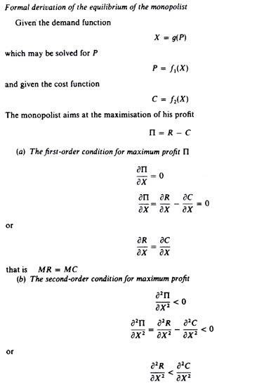
A monopolist maximizes his short-term profits if the following two conditions are met first, MC equals Mr. Secondly; the slope of MC is larger than that of Mr at the intersection.

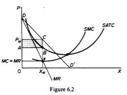
In Figure 6.2, the equilibrium of the monopoly is defined by the point θ at which MC intersects the MR curve from below. Thus, both conditions of equilibrium are met. The price is PM and the quantity is XM. Monopolies realize excess profits equal to shaded areas APM CB. Please note that the price is higher than Mr

In pure competition, the company is the one who receives the price, so it’s only decision is the output decision. The monopolist is faced with two decisions: to set his price and his output. But given the downward trend demand curve, the two decisions are interdependent.

Monopolies set their own prices and sell the amount the market takes on it, or produce an output defined by the intersection of MC and MR and are sold at the corresponding price. An important condition for maximizing the profits of monopolies is the equality of the MC and the MR, provided that the MC cuts the MR from below.

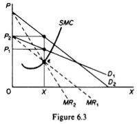
We can now revisit the statement that there is no unique supply curve for the monopolist derived from his MC. Given his MC, the same amount could be offered at different prices depending on the price elasticity of demand. This is graphically shown in Figure 6.3. Quantity X is sold at price P1 if demand is D1, and the same quantity X is sold at price P2 if demand is D2.  

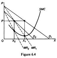
  So there is no inherent relationship between price and quantity. Similarly, given the monopolist MC, we can supply various quantities at any one price, depending on the market demand and the corresponding MR curve. Figure 6.4 illustrates this situation. The cost condition is represented by the MC curve. Given the cost of a monopolist, he would supply 0X1 if the market demand is D1, then p at the same price, and only 0X2 if the market demand is D2 B.Long-term equilibrium:

In the long run the monopolist will have time to expand his plants or use his existing plants at every level to maximize his profits. However, if the entry is blocked, the monopolist does not need to reach the optimal scale (that is, the need to build the plant until the minimum point of LAC is reached), neither does the guarantee that he will use his existing plant at the optimum capacity. What is certain is that if he makes a loss in the long run, the monopolist will not stay in business.

He will probably continue to earn paranormal benefits even in the long run, given that entry is banned. But the size of his plant and the degree of utilization of any plant size depends entirely on the market demand. He may reach the optimal scale (the minimum point of Lac), stay on the less optimal scale (the falling part of his LAC), or exceed the optimal scale (expand beyond the minimum LAC), depending on market conditions.

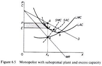
Figure 6.5 shows when the market size does not allow the monopolist to expand to the minimum point of Lac. In this case, not only is his plant not optimal (in the sense that the economy of full size is not depleted), but also the existing plant is not fully utilized. This is because on the left of the minimum point of the LAC, the SRAC touches the LAC at its falling part, and the short-term MC must be equal to the LRMC. This happens in e, but the minimum LAC is b,and the optimal use of the existing plant is a. Since it is utilized at Level E', there is excess capacity.                                                                Finally, figure 6.7 shows a case where the market size is large enough for a monopolist to build an optimal plant and be able to use it at full capacity.

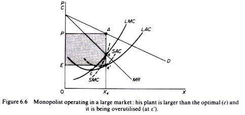
In Figure 6.6, the scale of the market is so large that monopolists have to build plants larger than the optimal ones to maximize output and over-exploit them. This is because to the right of the minimum point of LAC, SRAC and LAC is tangent at the point of positive slope, and SRMC must be equal to LAC. Thus, plants that maximize the profits of monopolies are, firstly, larger than the optimal size, and secondly, they are over-utilized, which leads to higher costs. This is often the case with utility companies operating at the state level.     

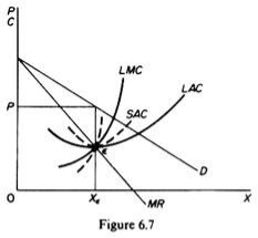
It should be clear that which of the above situations will appear in a particular case will depend on the size of the market (given the technology of monopolists). There is no certainty that monopolies will reach their optimal size in the long run, as is the case with purely competitive markets. In Monopoly, there is no market force similar to those of pure competition that will lead companies to operate at optimal plant size in the long run (and utilize it at its full capacity).

Price determination:

A monopolistic firm is a price-maker, not a price-taker. Therefore, a monopolist can increase or decrease the price. Also, when the price changes, the average revenue, and marginal revenue changes too. Take a look at the table below:

Let’s look at the revenue curves now:

As you can see in the figure above, both the revenue curves (Average Revenue and Marginal Revenue) are sloping downwards. This is because of the decrease in price. If a monopolist wants to increase his sales, then he must reduce the price of his product to induce:

• The existing buyers to purchase more

• New buyers to enter the market

Hence, the demand conditions for his product are different than those in a competitive market. In fact, the monopolist faces demand conditions similar to the industry as a whole.

Therefore, he faces a negatively sloped demand curve for his product. In the long-run, the demand curve can shift in its slope as well as location. Unfortunately, there is no theoretical basis for determining the direction and extent of this shift.

Talking about the cost of production, a monopolist faces similar conditions that a single firm faces in a competitive market. He is not the sole buyer of the inputs but only one of the many in the market. Therefore, he has no control over the prices of the inputs that he uses.

Role of time element in determination of price are given below:

Time plays an important role in the theory of volume, i.e., price determination because supply and demand conditions are affected by time.

Price during the short-period can be higher or lower than the cost of production, but in the long-period price will have a tendency to be equal to the cost of production.

The relative importance of supply on demand in the determination of price depends upon the time given to supply to adjust itself to demand.

To study the relative importance of supply or demand in price determination, Prof. Marshall has divided time element-into three categories:

(a) Very short period or market period.

(b) Short period.

(c) Long period.

(a) Very short period (determination of market price):

Market period is a time period which is too short to increase production of the commodity in response to an increase in demand. In this period the supply cannot be more than existing stock of the commodity.

The supply of perishable goods is perfectly inelastic during market period. But non-perishable goods (durable goods) can be stored.:

Therefore, the supply curve of non-perishable goods above reserve price has a positive scope at first but becomes perfectly inelastic after some price level.

The reserve price y depends upon-(i) cost of storing, (ii) future expected price, (iii) future cost of production, and (iv) seller’s need for cash we will discuss the determination of market price by taking a perishable commodity and determination of market price is illustrated.

DD is the original demand curve and SS the market period supply curve. The demand curve DD (perfectly inelastic) cuts the supply curve SS at point E. Point E, is the equilibrium point and equilibrium price is determined at OP, level.

Increase in demand shifts the demand curve to D,D and the price also increased to OP,. Decrease in demand shifts the demand curve downward to D2D2 and the price too falls to OP It is, thus, clear that in market period price fluctuates with change in demand conditions.

(b) Price determination is short period:

In the short period fixed factors of production remain unchanged, i.e., productive capacity remains unchanged.

However, in the short period supply can be affected by changing the quantity of variable factors.

In other words, during the short period supply can be increased to some extent only by an intensive use of the existing productive capacity.

Therefore, the supply curve in the short-run slopes positively, but the supply curve is less elastic. Determination of price in the short-run is illustrated.

SS is the market period supply curve and SRS is short-run supply curve. The original demand curve DD cuts both the supply curves at E, point and thus OP, price is determined.

Increase in demand shifts the demand curve upward to the right to D,D,. Now with the increase in demand the market price (in market period) rises at once to OP3 because supply remains fixed. But in the short-run supply increases. Therefore, in the short-run price will cuts the SRS curve. If demand decreases opposite will happen.

(c) Price determination in long period (Normal Price):

In the long period there is enough time for the supply to adjust fully to the changes in demand.

In the long period all factors are variable. Present firms can increase on decrease the size of their plants (productive capacity).

The new firms can enter the industry and old firms can leave the market. Therefore, long-period supply curve has a positive slope and is more elastic than short period supply curve.

The shape of supply curve of the industry depends upon the nature of the laws of returns applicable to the industry. Price determination in the long period is illustrated.

DD is the original demand curve and LS is the long period supply curve of the industry. Demand curve DD and supply curve LS both intersect each other at E point and OP price is determined.

This price will be equal to minimum average cost (AC) of production because in the long period firms under perfect competition can only earn normal profits. Suppose these are permanent increase in demand.

With the increase in demand, the demand curve shifts to D1,D1. As a result of increase in demand the price in the market period and short period will rise.

Due to increase in price present firms will earn above normal profit. Therefore, new firms will enter into market in the long period.

As a result of it supply will increase in the long period. In the long period price will be determined at OP1, level because at this price demand curve D1 D2 cuts the LS curve at E2 point..

Price OP1, is greater than previous price OP1, because the industry is an increasing cost industry. This new higher price will also be equal to minimum average cost of production.

Key takeaways –

3.3 Monopolistic Competition- Features and Equilibrium

Monopolistic competition:

In Monopolistic competition there are large numbers of buyers and sellers which do not sell homogenous product unlike perfect competition. This is more realistic in the real world. Monopolistic competition occurs when an industry in which many firms selling products that are similar but not identical.

Monopolistic competitions try to differentiate its product. Thus it is closely related to business strategy of brand differentiation. In monopolistic competition heavy advertising and marketing is common among firms.

Monopolistic competition combines element of both monopoly and perfect competition. All firms in monopolistic competition relatively have low market power and they are all market makers.

Monopolistic competitive market -

.

Features: 

2.     Many firms – there are many firms in each product group. A product group is a "collection of similar products". Under monopolistic market, each firms has a small market share.  This gives each firm a freedom to set price and each firm action have negligible impact on the market. A firm can cut the price to increase sale without any fear. As its action will not prompt retaliatory responses from competitors.

3.     Freedom of entry and exit - Like perfect competition, under monopolistic competition the firms can freely enter or exit. When the existing firms makes super-normal profits, then new firms will enter. The entry of new firms leads to increase the supply of goods and services and this would reduce the price and thus the existing firms will be left only with normal profits. Similarly, if the existing firms are incurring losses, some of the firms will exit. This will reduce the supply which result decrease in price and the existing firms will be left only with normal profit.

4.     Independent decision making – under monopolistic market, each firm can independently sets the terms and conditions of exchange for its product. The firm does not consider how their decision will have impact on competitors. In other words, each firm feels free to set prices and prompting heightened competition.

5.     Market power – under monopolistic competition, the firms have low degree of market power. Market power means that the firm has control over the terms and conditions of exchange for its product. All firms under monopolistic competition are price makers. A firm can raise the prices of products and services without losing all its customers base. The firm can also lower prices without any effect on the competitors. Since the firm have relatively low market power, there is no barrier to entry.

Monopolistic competition price and output decision-equilibrium:

Under monopolistic competition a firm can some extent independently control the supply and price of the product. The demand curve is stable and slightly downward slope

A monopolistic competitor creates output at which the marginal cost is equal to marginal revenue. The price is greater than marginal cost.

Short run-

In short run, the firm attains its equilibrium where marginal revenue equals marginal cost and the price is set according to its demand curve. Thus when MR=MC, profits are maximized

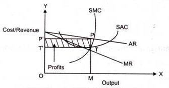
In the above fig,

In the above figure we can see that at output OM, MR intersects SMC. Here  price is OP’ (which is equal to MP). Thus P is the point on AR curve, which is price. PT is the supper normal profit per unit output, is the difference between the average revenue and average cost.

Long run-

In the long run due to the possibility of new firms entering the industry the price under monopolistic competition becomes equal to long-run average cost giving only normal profits. So, no firm under monopolistic competition can make excess profit or loss in the long run.

When the new firm start supplying , the price would fall. Thus the AR curve shifts from right to left and supernormal profits are replaced with normal profits. The long run equilibrium is achieved when average revenue is equal to average cost.

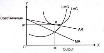
In the above fig we can see that, at pointP, AR curve touches the average cost curve (LAC) as a tangent. P is the equilibrium at price MP and output OM.

At MP average cost is equal to average revenue. Therefore, in long run, the profit is normal. The conditions (MR=MC and AR=AC) result in attaining equilibrium in long run.

Key takeaways –

3.4           Oligopoly: Concept and Features

In oligopoly there are small numbers of firms in the market. As per the norms, oligopoly consist of 3 -5 dominant firms. The firms can compete with each other or collaborate to earn more profits. Here the buyers are more than the sellers.

Features:

Key takeaways-  

3.5           Duopoly: Concept and Features

Duopoly is a limiting case of oligopoly, in the sense that it has all the characteristics of oligopoly except the number of sellers which are only two increase of duopoly as against a few in oligopoly. The main distinguishing feature of duopoly (and also of oligopoly) from other market situating is that the sellers’ decisions are not independent of each other. A change in price and output by our seller affect the former, and now the former may have to react. This process of action- reaction of the sellers may continue. This when a duopolist (or an oligopolist) takes any policy decision he also takes into account the reactions of his rivals. That is, such a market situation is characteristics by the mutual interdependence in policy-making.

Features:

Key takeaways-

3.6           Comparison of Perfect and Imperfect Competition

Key takeaways –

References