UNIT 4
Factor pricing
Marginal Productivity:
The oldest and most significant theory of factor pricing is the marginal productivity theory. It is also known as Micro Theory of Factor Pricing.
It was propounded by the German economist T.H. Von Thunen. But later on many economists like Karl Mcnger, Walras, Wickstcad, Edgeworth and Clark etc. contributed for the development of this theory.
“The distribution of income of society is controlled by a natural law, if it worked without friction, would give to every agent of production the amount of wealth which that agent creates.” – J.B. Clark
“The marginal productivity theory contends that in equilibrium each productive agent will be rewarded in accordance with its marginal productivity.” - Mark Blaug.
Assumptions of the Theory:
The main assumptions of the theory are as under:
1) Perfect Competition:
The marginal productivity theory rests upon the fundamental assumption of perfect competition. This is because it cannot take into account unequal bargaining power between the buyers and the sellers.
2) Homogeneous Factors:
This theory assumes that units of a factor of production are homogeneous. This implies that different units of factor of production have the same efficiency. Thus, the productivity of all workers offering the particular type of labour is the same.
3) Rational Behaviour:
The theory assumes that every producer desires to reap maximum profits. This is because the organizer is a rational person and he so combines the different factors of production in such a way that marginal productivity from a unit of money is the same in the case of every factor of production.
4) Perfect Substitutability:
The theory is also based upon the assumption of perfect substitution not only between the different units of the same factor but also between the different units of various factors of production.
5) Perfect Mobility:
The theory assumes that both labour and capital are perfectly mobile between industries and localities. In the absence of this assumption the factor rewards could never tend to be equal as between different regions or employments.
6) Interchangeability:
It implies that all units of a factor are equally efficient and interchangeable. This is because different units of a factor of production are homogeneous, since they are of the same efficiency, they can be employed inter-changeable, and e.g., whether we employ the fourth man or the fifth man, his productivity shall be the same.
7) Perfect Adaptability:
The theory takes for granted that various factors of production are perfectly adaptable as between different occupations.
8) Knowledge about Marginal Productivity:
Both producers and owners of factors of production have means of knowing the value of factor’s marginal product.
9) Full Employment:
It is assumed that various factors of production are fully employed with the exception of those who seek a wage above the value of their marginal product
10) Law of Variable Proportions:
The law of variable proportions is applicable in the economy.
The Amount of Factors of Production should be Capable of being Varied:
It is assumed that the quantity of factors of production can be varied i.e. their units can either be increased or decreased. Then the remuneration of a factor becomes equal to its marginal productivity.
11) The Law of Diminishing Marginal Returns:
It means that as units of a factor of production are increased the marginal productivity goes on diminishing.
12) Long-Run Analysis:
Marginal productivity theory of distribution seeks to explain determination of a factor’s remuneration only in the long period.
Theory of Distribution:
Distribution in economics refers to the way total output, income, or wealth is distributed among individuals or among the factors of production (such as labour, land, and capital). In general theory and the national income and product accounts, each unit of output corresponds to a unit of income. One use of national accounts is for classifying factor incomes and measuring their respective shares, as in National Income. But, where focus is on income of persons or households, adjustments to the national accounts or other data sources are frequently used. Here, interest is often on the fraction of income going to the top (or bottom) x percent of households, the next y percent, and so forth (say in quintiles), and on the factors that might affect them.
THEORIES OF DISTRIBUTION
Some important definitions of ‘Distribution’ are as follows:
According to Prof. Nicholson – “Distribution refers to the sharing of wealth of a nation among the different classes.”
Prof. Chapman has said that – “The Economics of Distribution accounts for the sharing of the wealth produced by a community among the agents or the owners of agents which have been active in its production.”
According to Prof. Cannon – “Distribution like production is a social phenomenon. In production we study the creation of social income and in distribution we study its distribution in one case we regard it as national output and in the other as national dividend.”
According to Prof. Seligman – “All wealth that is created in society finds its way to the final disposition of the individual, through certain channels or sources of income, this process is called distribution.” Thus, the theory of distribution deals with the distribution of income. It seeks to explain the principles governing the determination of factor like rewards—rent, wages, interest and profits—i.e., how prices of the factors of production are set. The theory of distribution thus states how the product is functionally distributed among the co-operating factors in the process of production.
Functional Distribution:
Functional distribution refers to the distinct share of the national income received by the people, as agents of production per Unit of time, as a reward for the unique functions rendered by them through their productive services. These shares are commonly described as wages, rent, interest and profits in the aggregate production. It implies factor price determination of a class of factors. It has been called as “Macro” concept.
Personal Distribution:
Personal distribution on the other-hand, is a ‘Micro Concept’ which refers to the given amount of wealth and income received by individuals in society through their economics efforts, i.e., individual’s personal earnings of income through various sources
The concept of equality and inequality of income distribution and social justice is basically concerned with the personal distribution of income. Taxation measures are designed to influence personal distribution of income and wealth in a community.
The theory of distribution deals with functional distribution and not with personal distribution of income. It seeks to explain the principles governing the determination of factor rewards like—rent, wages, interest and profits, i.e., how prices of the factors of production are set.
Key takeaways –
Meaning:
David Ricardo defined rent as “that portion of the produce of the earth which is paid to the land lord for the use of original and indestructible powers of the soil”. Thus, rent is only a payment for the use of land. The following are the theories of rent: (i) Ricardian Theory of Rent, and (ii) Modern Theory of Rent.
Ricardian theory of rent:
David Ricardo, an English classical economist, first developed a theory in 1817 to explain the origin and nature of economic rent. Ricardo used the economic and rent to analyse a particular question. In the Napoleonic wars (18.05-1815) there were large rise in corn and land prices.
He defined rent as “that portion of the produce of the earth which is paid to the landlord for the use of the original and indestructible powers of the soil.”
Assumption:
Reasons for existence of rent:
Let us assume that there are four types of land, classified based on its fertility, viz., A, B, C and D. A is the most fertile land and D is the least fertile land. People from the neighboring place come in batches to settle on the land. The first batch of people will naturally cultivate the most fertile land, i.e., A grade land. Let us assume that one dose of labour and capital on ‘A’ quality land yields 20 quintals of paddy per acre. Then, the second batch of settlers has two alternatives - either to cultivate B quality land, which is free, or to take ‘A’ quality land on rent from the first batch. It is obvious that the rent payable on the ‘A’ quality land would be equal to the differences in the fertilities of A and B quality lands. Let us assume that one dose of labour and capital applied to ‘B’ quality land yields 18 quintals of paddy. Now the rent is equal to 2 quintals, i.e., 20-18 quintals of paddy, because this represents the difference between the fertilities of the two types of lands.
Return from different qualities of land | ||||
labour and capital | Returns (in quantils of paddy per acre) | |||
| A | B | C | D |
1 | 20 | 18 | 16 | 14 |
2 | 18 | 16 | 14 | 12 |
3 | 16 | 14 | 12 | 10 |
4 | 14 | 12 | 10 | 8 |
Even if the second batch decides not to take up A quality land on rent, rent would still arise on ‘A’ quality land. Since the market price of paddy will be equal to the cost of production at ‘B’ quality land, ‘A’ quality land will have a surplus over ‘B’ quality land. The surplus return for A quality land arises due to its superior fertility in comparison with the ‘B’ quality land. Suppose, if 10 doses of labour and capital are available, rent from various qualities of land will be:
Rent of A grade land = Total quantity of produce - Total cost
= 68 – 56 = 12 quintals
Rent of B grade = 48 - 42 = 6 quintals
Rent of C grade = 30 - 28 = 2 quintals
Rent of D grade = 14 - 14 = 0 (no rent)
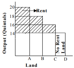
In this example, D quality land is the marginal or no-rent land, because it earns no rent. Thus, rent arises on account of natural differential advantages of a piece of land over the marginal land. The natural differential advantages may be due to either superior quality of land or its better situation.
Criticisms of the Ricardian Theory of Rent :
According to Ricardo, rent is due to the original and indestructible powers of the soil. But the fertility of the soil can be increased through manuring. Likewise, fertility of the soil can be destroyed through continuous cultivation without manuring.
In a thickly populated country, even the most inferior land yields rent and there is no marginal land in those countries. Thus, rent is not due to fertility, but to the scarcity of land.
Modern Theory of Rent:
Economists like Alfred Marshall, Joan Robinson criticized Ricardian theory of Rent and put forward a new approach. They believed that rent does not arise due to fertility of the land rather it arises due to Scarcity of a factor. Although land is free gift of nature but it is not free for a firm or enterprise. They have to pay for its usage and the price is decided by the scarcity i.e. more scare the factor more price for it. So the availability of the factor affects its price. Here the concept of opportunity cost comes in play. Opportunity cost is the value of next best available alternative .A Factor needs to be paid minimum amount equal to its opportunity cost. Remember it is the minimum amount i.e. the lowest limit, actual amount may be much higher.
The actual amount to be paid depends on the scarcity and availability of that factor. If the factor is scare i.e. less available then the buyer has to pay more amount (Price) for that factor than its opportunity cost. This extra payment is nothing but Rent which depends on scarcity of a factor. Similarly for less scare factor buyer may pay an amount equal or slightly higher than its opportunity cost.
So rent is the extra payment over the opportunity cost (Minimum cost which has to be incurred). The scare factor attracts more rent as the difference in the opportunity cost and actual rent paid is more. Ricardo in his theory assumed that rent arises only on land but the advocates of Modern theory of rent believed that rent can arise on any factor of production.
Suppose an IT professional is working in firm A for a monthly package of Rs.one lakh. With the growing IT sector, the demand for IT professionals will increase. Now firm B offers him a monthly package of Rs. two lakh and he accepts the same.
Opportunity cost in above example = 1,00,000
Actual earning of factor = 2,00,000
Rent= Actual earning- Opportunity cost i.e. 200000-100000=100000
The rent of one lakh is result of scarcity of IT professionals i.e. demand of IT professionals are more than its supply as a result their price increases.
The scarcity of factor can be shown with the help of its Supply curve. If the factor is highly scare its supply curve will be vertical to the X axis or perfectly inelastic showing zero opportunity cost and whole amount as rent. On the other hand if the factor is not scare at all supply curve will be horizontal to the X axis or perfectly elastic one showing that the opportunity cost is equal to actual amount and hence Zero rent. So the shape of supply curve is the indicator of scarcity of the factor.
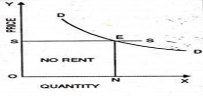
The above diagram shows the situation of no Rent. As you can see the supply cure is perfectly elastic indicating that the factor is not scare at all. Here the opportunity cost is same as the actual amount spent i.e. the minimum amount of opportunity cost is equal to the actual earning of the factor.

The above diagram shows the case of completely scare factor in which the whole earning is the amount of rent. Here the opportunity cost is zero and supply curve is perfectly inelastic. So whatever the demand for the factor determine its price and the whole amount represents the rent which is OPSE in the above diagram.
Concept of Quasi Rent:
Quasi rent is the earning of capital equipments such as machineries, buildings etc., which are inelastic in supply, in short run. According to Marshall, the quasi rent is only a temporary surplus, which is enjoyed by the owner of the capital equipments in the short run. This is due to the increase in its demand and it will disappear in the long run, if supply of the capital equipment is increased in response to the increased demand. The quasi rent is also defined as the excess of total revenue earned in the short run over and above the total variable costs. Thus, Quasi Rent = Total Revenue Earned minus Total Variable Costs.
Ricardian rent is a payment made for the use of land whereas quasi-rent is a payment for manmade factors such as buildings, machineries, etc. Ricardian rent Wage Fund Rate of Wages = Number of Workers exists both in short run and long run because supply of land is fixed in long run. But quasi rent is only a temporary earning due to increased demand.
Key takeaways –
Backward Bending Supply Curve of Labour
Role of Collective Bargaining in Wage Determination
Meaning:
Wage is defined as the price paid for the services rendered by the labourer in the production process. If wages are paid according to the amount or quantum of work done, it is called piece-wage. E.g. wage for weeding in one acre of paddy field. If wages are paid to a labourer who works for a fixed period of time, it is known as time wage. E.g. wage for weeding per labourer per day.
When payment is made in terms of cash or money, it is known as money wage or nominal wage. Real wage refers to the income of a worker in terms of real benefit. It refers to the amount of necessaries, comforts, and luxuries that a labourer can obtain in return for his services. Real wage refers to the purchasing power of money earned by the labourer or wages paid in terms of quantity of commodities. The standard of living of a labourer depends on his real wage.
Types of wages-
a) Minimum Wages :
According to Fair Wages Committee, “Minimum Wages should provide not only for the bare necessities of a worker. It should also provide for the maintenance of efficiency of the worker. From this point of view, minimum wages must be sufficient to provide for all requirements of education, health and other essential amenities”. Minimum Wages means the minimum payment to worker so that he may be able in providing for basic needs for himself and his family members and to maintain his working efficiency only.
b) Money Wages:
Nominal or money wages are the payments done to workers in money form and do not take account of inflation rates and any other market conditions. Money wages do not take into consideration the purchasing power and the employee receives the amount that is promised to him when he/she is hired. For example, if a worker receives Rs15 per hour from their organization in exchange of the services or labor provided, then that is the nominal wage. The basic determinants of the nominal wages would be the government regulations and the organization’s compensation policy within its capacity.
c) Real Wages:
Real wages are the type of wages that take inflation rates into consideration. These wages determine the purchasing power the individual has and the amount of goods or services the individual can purchase given the current market conditions. In other words, it can also be defined as the actual amount of goods and services the employee can purchase with the payments given after inflation has been considered. Real wages indirectly affect nominal wages as the real wage rises employees can easily demand for more money wages.
d) Subsistence Wages:
Wages tend to remain at the subsistence level. Wages paid to workers is just sufficient to fulfill their basic needs. Workers don’t have surplus income. If wages rises above this level, this leads to an increase in the population because the increased prosperity of workers will encourage the workers to marry sooner and increase population. This will increase labor supply. The increased competition among workers for employment causes wages to fall again to the subsistence level.
e) Fair Wages:
Prof. Pigou, “Fair wages is the wages which is paid at the rate which is being paid to the workers of same status in the enterprises of the same type and of near-by areas”. Fair wages is more than minimum wages. Fair wage is determined after considering several factors such as the wages paid for similar work in other trades, etc. fair wage is determined between the lower and the upper limits. The lower limit of wage is the minimum wage and the upper limit is the capacity of the industry to pay.
Backward Bending Supply Curve of Labour:
A typical supply curve shows an increase in supply as wages rise. It slopes from left to right.
However, in labour markets, we can often witness a backward bending supply curve. This means after a certain point, higher wages can lead to a decline in labour supply. This occurs when higher wages encourage workers to work less and enjoy more leisure time.
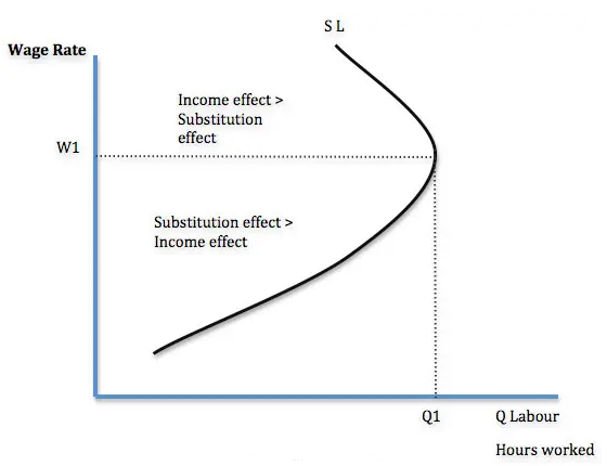
There are two effects related to determining supply of labour-
Role of Collective Bargaining in Wage Determination:
Collective bargaining is a process of negotiation between employers and a group of workers aimed at agreements to regulate working salaries, working conditions, benefits, and other aspects of workers' compensation and rights .
The interests of the workers are commonly presented by representatives of a trade union to which the workers belong.
The collective agreements reached by these negotiations usually set out wage scales, working hours, training, health and safety, overtime, grievance mechanisms, and rights to participate in workplace or company affairs.
A collective agreement functions as a labour contract between an employer and one or more unions.
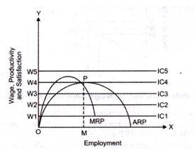
The above figure shows the determination of wage rate with the help of the collective bargaining process.
ARP represents the average net revenue productivity curve and MRP represents marginal net revenue productivity curve. IC1, IC2, IC3, IC4, and IC5 show indifference curves at different wage rates with respect to the satisfaction of trade unions. It can be seen that an increase in the wage rate would result in the increase of satisfaction level of trade unions.
In this case, trade union would prefer the wage rate at point P where indifference curve is tangent to ARP. At point P, the wage rate is OW4 and number of labor is OM. In case the wage rates goes up from OW4, then the employer would suffer losses and he/she needs to close his/her unit.
Therefore, it is not beneficial for the employer as well as for the union. This makes OW4 an upper limit for deciding on the wage rate.
Key takeaways –
Interest meaning:
Interest is a payment made by a borrower to the lender for the money borrowed and is expressed as a rate percent per year. Interest implies the return to capital as a factor of production. But for all practical purposes, “interest is the price of capital.” Capital as a factor of production, in real terms, refers to the stock of capital goods (machinery, raw-materials, factory plant etc.).
As Prof. Marshall has said – “The payment made by borrower for the use of a loan is called interest”.
Loanable fund theory of interest:
According to this theory, rate of interest is determined by demand and supply of loanable funds. The supply of loanable funds consists of (i) savings of people out of their disposable income, (ii) dishoarding by people from past savings, (iii) disinvestments and (iv) bank credit. The supply of loanable fund is positively related to the rate of interest and hence, the supply curve of loanable funds is upward sloping. In other words, larger amount of loanable funds will be available at higher rates of interest and vice-versa.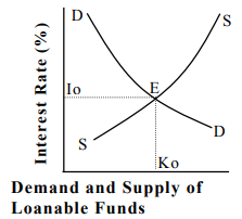
Loanable funds are demanded for the following three purposes:
The demand for loanable funds is inversely related to rate of interest. So the demand curve of loanable funds is inversely period of time in the case of long-term loan. So he expects higher interest rate for such loans. The equilibrium interest rate gets determined at the point (E) where supply of loanable funds equals demand for loanable funds, i.e., at equilibrium point the demand and supply curves cut each other. Thus, this theory states that savings of people depend upon the interest rate. But Keynes has shown that savings of people depend upon money income and their preference to keep liquid cash.
Liquidity preference theory:
The ‘real’ factors of the supply of saving and the demand for investment are the determinants of the equilibrium interest rate in the classical model. Whereas in the Keynesian analysis, determinants of the interest rate are the ‘monetary’ factors alone.
As the determinants of interest rate, Keynes’ analysis concentrates on the demand for and supply of money. According to Keynes, the rate of interest is purely “a monetary phenomenon.” The price paid for borrowed funds is the interest. The rate of interest in the Keynesian theory is determined by the demand for money and supply of money.
Demand for money
The desire for demand for money arises because of three motives:
Transaction Demand for Money: For day to day transaction money is needed. Money is demanded as there is gap between the receipt of income and spending. Income is earned at the end of week or month but individuals income are spent to meet day to day transaction. Throughout the period spending are made but income are received after a period of time. To finance the transaction individual needs active balance in the form of cash. This is known as transaction demand for money. To meet day to day transaction people with higher income keep more liquid money. Transaction demand for money is an increasing function of money income.
Tdm= f (Y)
Where,
Pdm = f (Y).
2. Speculative Demand for Money: The speculative motive refers to the desire to hold one’s assets in liquid form to take advantages of market movements regarding the uncertainty and expectation of future changes in the rate of interest.
Sdm = f (r) Where, Y is the rate of interest.
3. Total demand for money - The total demand for money (DM) is the sum of all three types of demand for money.
That is, Dm = Tdm + Pdm + Sdm.
The demand for money has a negative slope because of the inverse relationship between the speculative demand for money and the rate of interest.
Key takeaways –
Meaning:
Profit is the reward to an entrepreneur for the functions he renders in productive activity. Out of the income earned by the farm, land owner is paid rent, labourer is paid wage and capitalist is paid interest. Whatever is left over goes to the entrepreneur as profit. Hence, profit is also called a residual income
Risk and Uncertainty Theory of Profit:
Risk Bearing Theory of Profit -
According to Professor Hawley, profits are the rewards for risk taking, which is an important function of an entrepreneur. Production is carried on in anticipation of demand. However, the risks due to theft, accidental damages, price changes (which may again be due to change in fashion, tastes, preferences, etc), labour strike and so on may cause losses. Hence, the entrepreneur has to reduce these risks wherever it is possible. The risk taking is an unpleasant work, though an essential job, for which the entrepreneur has to be suitably rewarded. That reward is called profit. However, there are certain risks for which the consequences are not known well in advance and such risks cannot be insured against. The remuneration for known risks is not profit. Profit arises on account of assumption of unknown risks and it is explained by the uncertainty theory. 3.
Uncertainty-Bearing Theory of Profit -
This theory was propounded by F.H. Knight. Knight divided risks into (i) foreseeable risk-a risk that can be foreseen by the entrepreneur and (ii) unforeseeable risk-a risk, which cannot be foreseen by the entrepreneur. Knight calls this unforeseeable risk as uncertainty. According to Knight, profit does not arise on account of foreseeable risk, since such risks can be insured. Hence, risk taking is not the function of the entrepreneur, but of the insurance companies. Profit, according to Professor knight, is due to non-insurable risk (or, unforeseeable risk). A loss due to fire accident in a factory is an insurable risk. A few cases of non-insurable risks are: (i) Loss due to labour strike, (ii) loss due to heavy competition from rival companies, (iii) Loss due to changes in tastes and preferences of the consumer which in turn would result in low demand for the product. It is the primary function of the entrepreneur to anticipate and provide alternative arrangements to tackle non-insurable risks or uncertainties. Thus, profit is paid to the entrepreneur for his ability to bear uncertainty and not for risk-taking.
Dynamic Theory of Profit -
The dynamic theory of profit developed by J. B. Clark suggests that profit is generated in a society which is dynamic in nature. The dynamic nature of a society means that the population, size of capital, level of output, taste and preferences of people of that society are changing. All these changes cause the gap between price and unit cost. Profit arises when price exceeds unit cost. In a static society there are no changes in above variables and as a consequence the difference between price and unit cost does not arise. Thus profit is not generated in static society. There are risks or uncertainties associated with dynamic society and as a result of this it is difficult to forecast the future positions of price and output level. Thus entrepreneur claims profit as a reward of undertaking these risks or uncertainties in the dynamic society.
Innovation Theory of Profit -
The innovation theory of profit is developed by Schumpeter. The creation of new products or new process of production is called invention, while innovation is the commercial utilization of invention. Thus the innovator derives profit by utilizing commercially the newly invented products. An entrepreneur is said to be an innovator when he brings a new product for commercial purpose and can earn super normal profit. However, this super normal profit can be obtained only in the short run. This short run super normal profit induces others to introduce similar kind of products or similar process of productions and in the long run this additional profit will be reduced.
Key takeaways –
References