4.1 CURVE TRACING | unit 4 curve tracing 3

Back to Study material

M II

Unit-4

CURVE TRACING

BASIC DEFINITIONS

Convex Upwards: If the portion of the curve on both sides of point ‘A’ lies below the tangent at A, then the curve is convex upwards.
Convex Downwards:If the portion of the curve on both sides of point ‘A’ lies above the tangent at A, then the curve is convex downwards.
Singular points:An unusual point on a curve is called a singular point such as a point of inflexion, a double point, a multiple point, cusp, node or a conjugate point.
Point of Inflexion: The point that separate the convex part of a continuous curve from the concave part is called the point of inflexion of the curve. i.e. A point where the curve unusually crosses its tangent is called a point of inflexion.
Multiple Point:A point through which more than one branches of a curve pass is called a multiple point of the curve.
Double point: A point on a curve is called a double point, if two branches of the curve pass through it.If r branches pass through a point, the point is called a multiple point of rth order.
Node: A double point is called node if the branches of curve passing through it are real and the tangents at the common point of intersection are distinct.
Cusp: A double point is called Cusp if the tangents at that point to the two branches of the curve are coincident.
A Conjugate Point: A Point P is called a conjugate point on the curve if there are no real points on the curve in the vicinity of the point P. It is also called as an isolated Point.

4.1 CURVE TRACING

Tracing of Cartesian curves

The following rules will help in tracing a Cartesian curve.

Rule 1: Symmetry

(a) Symmetry about X-axis: If the equation of curve containing all even power terms in ‘y’ then the curve is symmetric about X-axis.

(b) Symmetry about Y-axis: If the equation of curve containing all even power terms in ‘x’

then the curve is symmetric about Y-axis

terms in ‘x’ and ‘y’ then the curve is symmetric about both axes.

(d) Symmetry in opposite quadrants: If the equation of curve remains unchanged when x and y are replaced by –x and –y respectively then the curve is symmetric in opposite quadrants.

(e) Symmetry about the line :If the equation of curve remains unchanged when x is replaced by y and y is replaced by x then the curve is symmetric about the line y=x.

(f) Symmetry about the line :If the equation remains unchanged when x is replaced by -y and y is replaced by - x then the curve is symmetric about the line y=-x.

Rule 2: Points of intersection

(a) Origin: If the equation of curve does not contain any absolute constant then the curve passes through the origin.

(b) Intersection with the co-ordinate axes:

Intersection with X-axis: put y=0 in the given equation and find the value of x.

Intersection with Y-axis: put x = 0 in the given equation and find the value of y.

Rule 3:Tangents

(a) Origin:If the curve passes through origin then the equations of the tangent at origin can be obtained by equating the lowest degree terms taken together to zero.

(b) Other points: Tofind nature of tangent at any point find at that point.

Case 1: If then tangent is parallel to X-axis.

Case 2: If then tangent is parallel to Y-axis.

Case 3: If then tangent makes acute angle with X-axis.

Case 4: If then tangent makes obtuse angle with X-axis.

Rule 4:Asymptotes:

(a) Parallel to X-axis: Asymptotes parallel to X-axis are obtained by equating the coefficient of highest degree term in x to zero.

(b) Parallel to Y-axis: Asymptotes parallel to Y-axis are obtained by equating the coefficient of highest degree term in y to zero.

Method 1: Let y=mx+c be the asymptote. The point of intersection with the curve f(x, y)=0 are given by f(x, mx+c)=0. Equate to zero the coefficients of two successive highest power of ‘x’, giving equations to determine m & c.

Method 2:

Let y= mx+c be the equation of asymptote.
Find by putting x=1 and y=m in the highest degree (n) terms of the equation.
Similarly find .
Solve =0 to determine m.
Find ‘c’ by the formula.
If the roots of m are equal, then find ‘c’ by .

Rule 5:Special points on the curve:Find out such points on the curve whose presence can be easily detected.

Rule 6:Region of absence of the curve: Findthe values of x(or y) where y(or x) becomes imaginary, then the curve does not exists in that region.

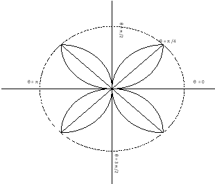
Q1) Trace the following curve:

Sol)

We check the following points for tracing of the above curve

Limit: i.e. total curve will lie inside the circle of radius ‘a’.

2. No. of loops: The curve contains 4 loops because is even.

3. Symmetry:

(i) About the line perpendicular to initial line i.e. the line:-

If we replace by and bythen the equation of the curve is remains unchanged.

The curve is symmetry about the line.

4. Pole:

(i) For .

Hence the curve passes through the pole.

(ii) Tangent at pole: If we put , then we get the tangent at

pole.

Putting in (1), we have

5. Asymptotes:No asymptotes.

6. Table values:


	0		0		0		0

It is clear that for, the value of r is zero therefore these are tangents at pole and for the value of r is maximum i.e. ‘a’. Hence, we get four loops at those points. Hence the approximate shape of the curve is as follows.

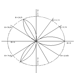
Q2) Trace the following curve:

Sol)

We check the following points for tracing of the above curve

Limit:i.e. total curve will lie inside the circle of radius ‘a’.

2. No. of loops:The curve contains 3 loops because is odd.

3. Symmetry:

(i) About initial line :-

If we replace by, then the equation of the curve is remains unchanged.

The curve is symmetry about the initial line.

4. Pole:

(i) For

Hence the curve passes through the pole.

(ii) Tangent at pole: If we put , then we get the tangent at pole.

Putting in (1), we have

5. Asymptotes:No asymptotes.

6. Table values:


			0		0		0	0

It is clear that for, the value of r is zero therefore these are tangents at pole and for the value of r is maximum i.e. ‘a’. Hence we get three loops at those points. Hence the approximate shape of the curve is as follows.

4.2 TRACING OF PARAMETRIC CURVES

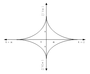
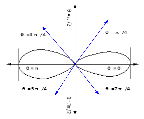
The following rules will help in tracing a Parametric curve

Rule 1:Limitations of the curve:

If possible, find the greatest and least values of x & y for a proper value of t.

Rule 2: Symmetry:

(a) Symmetry about X-axis: If ‘x’ is even and ‘y’ is odd w. r. t ‘t’

i.e. then the curve is symmetric about X-axis.

(b) Symmetry about Y-axis:

1. If ‘x’ is odd and ‘y’ is even w. r. t ‘t’

i.e. then the curve is symmetric about Y-axis.

2. For trigonometric functions if ‘x’ is odd and ‘y’ is even w. r. t ‘’

i.e. then the curve is symmetric about Y-

axis.

Symmetry in opposite quadrants: If ‘x’ and ‘y’ both are odd w. r. t ‘t’

i.e. then the curve is symmetric about opposite

quadrants.

Rule 3: Points of intersections:

It will pass through the origin if on putting t = 0 we obtain x = 0 and y = 0 . Also find

the points of intersection of the curve and the axes.

Rule 4: Nature of tangents:

2) Form the table of values of for different values of ‘t’.

Rule 5: Asymptotes and region:

1) Find asymptotes if any.

2) Find region of absence.

Q1) Trace the following curve:

Sol)

We have to trace the curve

or - - - - - - - - - (1)

We check the following points for tracing of the above curve

Limit:

2. Symmetry:

(i) About X- axis:

Since ‘x’ is even function and y is odd.

The curve is symmetry about x-axis.

(ii) About Y- axis:

If we replace by, then ‘x’ is odd function and ‘y’ is even function w.r.t. .

Hence the curve is symmetry about y-axis.

(iii) About Opposite Quadrant:

Since the curve is symmetry about both the axes.

It is symmetry about opposite quadrant.

3. Origin:

For.

Hence the curve does not pass through the origin.

4. Tangent:

5. Asymptotes:No asymptotes.

6. Table values:

It is clear that at, x-axis is tangent. Also when‘t’ increases from ‘0’ to the value of x decreases from ‘a’ toand the value of y increases from ‘0’ to. Hence, we get the curve in first quadrant. Since the curve is symmetry about Y-axis and X-axis. Hence the approximate shape of the curve is as follows:

Definition: Finding the length of an arc of the curves is called as Rectification.

Formulae of Rectification of plane curve for Cartesian equation:

Equation of curve

Formula in differential calculus

Formula Inintegral calculus

Ex1) Solve the following problems on Rectifications.

Show that for the curve and he perimeter of one of the loops is.

Sol)

Here the curve is symmetrical about X-axis and has two loops around X-axis between x = 0 and x = a.

We first integrate between x = 0 and x = a.

We first find arc length of the curve from origin to any point (x,y) on the curve.

Differentiating w.r.to x, the equation of curve, we get,

Now, =

Putting . When ,

Which is required result.

Now to get the perimeter of the loop, we put [Whenwhich gives the length of upper half of the loop].

Which is required length.

RECTIFICATION OF CURVES (Parametric and Polar Form)

4.3 RECTIFICATION OF CURVES

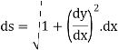
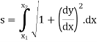
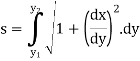
In this session we shall consider the application of integration to measure the length of an arc of Cartesian curve.

In this session we shall consider the application of integration to measure the length of an arc of parametric and polar curves.

Ex1) Find the total arc length of the curve.

Sol)

We have to find the total arc length of the curve

It can be written as

- - - - - - - - - - - - - - - - (1)

If we calculate the length of the arc in first quadrant, then we can find the total arc length of the curve multiplying by 4. In first quadrant varies form.