Unit-1
Discrete-time signals and systems
A complex exponential signal, whether in continuous time or in discrete time, is completely determined by its amplitude A, phase α, and frequency which can be F0 Hz (or Ω0 rad/sec) in continuous time or w0 radians in discrete time, as in the following expressions: X(t) =A ejα ejΩ0t = A ejα ej2πF0t
X[n] = A ejα ejw0n
When the signal is the superposition (ie sum) of two or more complex exponentials of different amplitudes and phases, we just add them in the plot and place them appropriately in frequency. So for example a sinusoidal signal, as
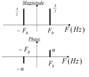
X(t) = A+ cos(2π F0t + α)
= (A/2) ejα ej2πF0t + (A/2) e-jα e-j2πF0t
is represented by two complex exponentials with frequencies F0 and -F0 respectively, as shown in figure. Notice the appearance of the negative frequency -F0 which corresponds to the complex exponential with the same amplitude and opposite phase.
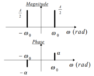
Similarly for the discrete time case. A discrete time sinusoid
X[n] = A cos(w0n +α) = (A/2) ejα ejw0n + (A/2) e-jα e-jw0n
Fig 1 Mapping of Analog Frequency and Digital Frequency
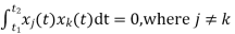
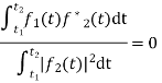
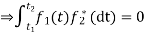
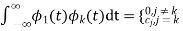
Orthogonality Let us consider a set of n mutually orthogonal functions x1(t), x2(t)... xn(t) over the interval t1 to t2. As these functions are orthogonal to each other, any two signals xj(t), xk(t) have to satisfy the orthogonality condition. i.e.
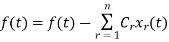
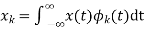
Let a function f(t), it can be approximated with this orthogonal signal space by adding the components along mutually orthogonal signals i.e.
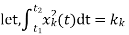
If
Where, Where, If
Basis Function
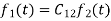
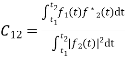
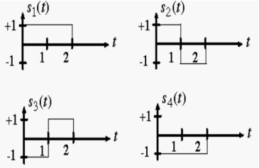
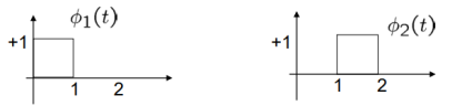
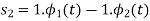
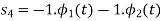
Example Consider the following signal set:
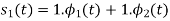
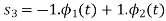
Solution: By inspection, the signals can be expressed in terms of the following two basis functions:
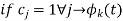
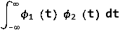
Note that the basis is orthogonal
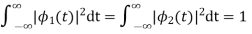
Also note that each these functions have unit energy
We say that they form an orthonormal basis.
Key takeaway Signal set
|


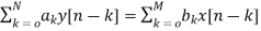
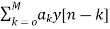
The general nth order difference equation is given as a0y[n]+ay[n-1]+….+aN-1y[n-N+1]+any[n-N]=b0x[n]+b1x[n-1]+….+bMx[n-M] The difference equation can be written as
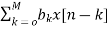
The output equation can be given as y[n] = The above difference equation can be solved by finding homogeneous and particular solution or by z transform method. Z transform is discussed in above section. Homogeneous Solution: Let x[n]=0
The solution to above equation will be of the form y[n] = rn Then solution will be of the form y[n] = p1 y[n]= p1n
Key takeaway
Examples Que) Find the homogenous solution for the difference equation y[n]- Sol: For homogeneous solution Y[n] = rn rn- rn-2(r2- Solving above equation we get r= Roots are distinct so the solution will be of the form y[n] = p1 y[n] = p12-n +
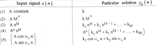
Particular Solution:
The complete solution of any difference equation is the sum of homogeneous solution and the particular solution. Que) For the difference equation find the particular solution x[n] = 3n y[n] = x[n]+ Sol: As x[n] = 3n From table the particular solution will be y[n] = k3n y[n] = x[n]+ k3nu(n) = 3nu(n)+ Finding k for n≥2 K 32 = 32+ 9k- k= 27/20 y[n]= |


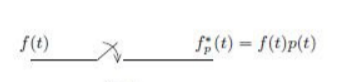
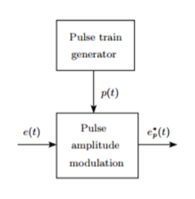
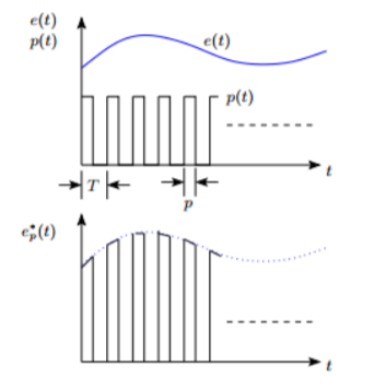
Sampling usually refers to conversion of continuous signal into short duration of pulses each pulse followed by a skip period when no signal is available. Below shown is a uniformly sampled signal. Following are two popular sampling operations: 1. Single rate or periodic sampling 2. Multi-rate sampling Figure below shows the structure and operation of a finite pulse width sampler, where 2(a) represents the basic block diagram and 2(b) illustrates the function of the same. T is the sampling period and p is the sample duration.
Figure 2 (a): Basic block diagram
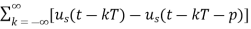
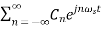
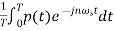
Figure 2 (b): Sampler output Finite pulse width sampler converts a continuous time signal into a pulse modulated or discrete signal. The most common type of modulation in the sampling and hold operation is the pulse amplitude modulation. The block diagram of sampler is shown above, having a pulse train of p seconds and sampling period of T seconds. p(t)= unit pulse train with period T p(t)= Us(t)=unit step function In frequency domain p(t) can be represented as p(t)=
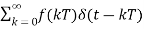
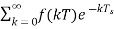
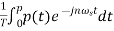
Cn= p(t)=1 for 0≤ t ≤p The output of the ideal sampler can be expressed as f*(t)= F*(s)= The output of the sampler can be approximated as Cn= =
Reconstruction process
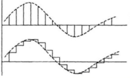
Fig 3 Sampled Data The sampled data signal is modified by the controller. The hold circuit than converts the signal to analog form. The simplest hold circuit is ZOH (zero order hold) in which the reconstructed signal acquires the same value as the last received sample for the entire sampling period. The basic sampler is shown in above figure (a) and output in figure (b). The high frequency signal present in the reconstructed signal is filtered by the controller elements which are the low pass in frequency behaviour. The first or higher order holds have no advantage over the ZOH. In the first order hold the last two signal samples are used to reconstruct the signal for the current sampling period.
Aliasing Aliasing can be referred to as “the phenomenon of a high-frequency component in the spectrum of a signal, taking on the identity of a low-frequency component in the spectrum of its sampled version.”
Key takeaway
Examples
1) The continuous-time signal x(t) = cos(200πt) is used as the input for a CD converter with the sampling period 1/300 sec. Determine the resultant discrete-time signal x[n].
Solution:
We know, X[n] =x(nT) = cos(200πnT) = cos(2πn/3) , where n= -1,0,1,2……
The frequency in x(t) is 200π rad/s while that of x[n] is 2π/3.
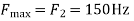
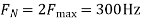
2) Determine the Nyquist frequency and Nyquist rate for the continuous-time signal x(t) which has the form of X(t) = 1+ sin(2000πt) + cos (4000πt)
Solution:
The frequencies are 0, 2000π and 4000π. The Nyquist frequency is 4000π rad/s and the Nyquist rate is 8000π rad/s.
3) Consider an analog signal
Solution. The frequency in the analog signal
The largest frequency is
The Nyquist rate is
4) The analog signal
Solution.
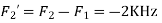
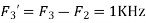
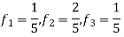
For Hence
So that normalizing frequencies are
The analog signal that we can recover is
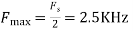
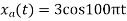
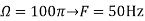
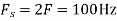
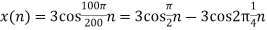
5) For given signal
Solution. a. The minimum sampling rate is
And the discrete time signal is
b. if
c. If Fs=75Hz , the discrete time signal is
d. For the sampling rate
So, the analog sinusoidal signal is
6) Suppose a continuous-time signal x(t) = cos (Ø0t) is sampled at a sampling frequency of 1000Hz to produce x[n]: x[n] = cos(πn/4). Determine 2 possible positive values of Ø0, say, Ø1 and Ø2. Discuss if cos(Ø1t) or cos(Ø2t) will be obtained when passing through the DC converter.
Solution: Taking T= 1/1000s cos(πn/4) =x[n] = x(nT) = cos (Ø0n/1000) Ø1 is easily computed as Ø1 = 250π
Ø2 can be obtained by noting the periodicity of a sinusoid:
Ø2 = 2250π
|


1.4.1 Sampling theorem
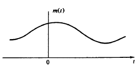
In sampling the signal m(t) is multiplied with periodic pulse train. Let M(ω) the spectrum of the input signal be band limited with the maximum frequency of fm as shown in figure 4.
Figure: 4 Spectrum of input signal
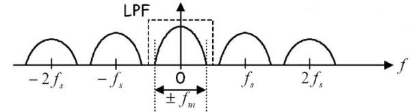
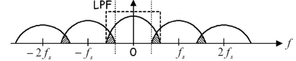
Figure: 5 (fs>2 fm) Figure: 6 (fs<2 fm) The frequency spectrum of this signal when impulse sampled is plotted in figure 5 (for fs>2 fm). In figure 6 for (fs<2 fm). From figure 5 and figure 6 we can conclude that as long as fs≥2fm the original signal is preserved in the sampled signal and can be extracted from it by the low pass filter. This is known as Shannon’s Sampling theorem. This theorem states that the information contained in a signal is fully preserved in the sampled form as long as the sampling frequency is at least twice the maximum frequency contained in the signal.
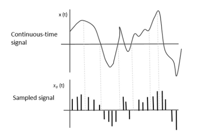
1.4.2 Nyquist rate. The following figure indicates a continuous-time signal x (t) and a sampled signal xs (t). When x (t) is multiplied by a periodic impulse train, the sampled signal xs (t) is obtained.
Fig 7 Sampled Signal To discretize the signals, the gap between the samples should be fixed. That gap can be termed as a sampling period Ts. Sampling Frequency=1/Ts=fs Where:
Sampling frequency is the reciprocal of the sampling period. This sampling frequency, can be simply called as Sampling rate. The sampling rate denotes the number of samples taken per second, or for a finite set of values. Suppose that a signal is band-limited with no frequency components higher than W Hertz. That means, W is the highest frequency. For such a signal, for effective reproduction of the original signal, the sampling rate should be twice the highest frequency. Which means, fS=2W Where:
This rate of sampling is called as Nyquist rate.
Key takeaway
|
References:
1. S. K. Mitra, “Digital Signal Processing: A computer based approach”, McGraw Hill, 2011.
2. A.V. Oppenheim and R. W. Schafer, “Discrete Time Signal Processing”, Prentice Hall, 1989.
3. J. G. Proakis and D.G. Manolakis, “Digital Signal Processing: Principles, Algorithms And Applications”, Prentice Hall, 1997.
4. L. R. Rabiner and B. Gold, “Theory and Application of Digital Signal Processing”, Prentice Hall, 1992.
5. J. R. Johnson, “Introduction to Digital Signal Processing”, Prentice Hall, 1992.
6. D. J. DeFatta, J. G. Lucas andW. S. Hodgkiss, “Digital Signal Processing”, John Wiley & Sons,1988.


