UNIT 1
Matrices and Determinants
Matrices have wide range of applications in various disciplines such as chemistry, Biology, Engineering, Statistics, economics, etc.
Matrices play an important role in computer science also.
Matrices are widely used to solving the system of linear equations, system of linear differential equations and non-linear differential equations.
First time the matrices were introduced by Cayley in 1860.
Definition-
A matrix is a rectangular arrangement of the numbers.
These numbers inside the matrix are known as elements of the matrix.
A matrix ‘A’ is expressed as-
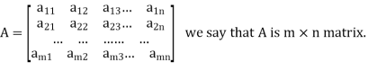
The vertical elements are called columns and the horizontal elements are rows of the matrix.
The order of matrix A is m by n or (m× n)
Notation of a matrix-
A matrix ‘A’ is denoted as-
A = 
Where, i = 1, 2, …….,m and j = 1,2,3,…….n
Here ‘i’ denotes row and ‘j’ denotes column.
Types of matrices-
1. Rectangular matrix-
A matrix in which the number of rows is not equal to the number of columns, are called rectangular matrix.
Example:
A = 
The order of matrix A is 2×3 , that means it has two rows and three columns.
Matrix A is a rectangular matrix.
2. Square matrix-
A matrix which has equal number of rows and columns, is called square matrix.
Example:
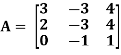
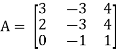
A = 
The order of matrix A is 3 ×3 , that means it has three rows and three columns.
Matrix A is a square matrix.
3. Row matrix-
A matrix with a single row and any number of columns is called row matrix.
Example:
A = 
4. Column matrix-
A matrix with a single column and any number of rows is called row matrix.
Example:
A = 
5. Null matrix (Zero matrix)-
A matrix in which each element is zero, then it is called null matrix or zero matrix and denoted by O
Example:
A = 
6. Diagonal matrix-
A matrix is said to be diagonal matrix if all the elements except principal diagonal are zero
The diagonal matrix always follows- 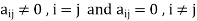
Example:
A = 
7. Scalar matrix-
A diagonal matrix in which all the diagonal elements are equal to a scalar, is called scalar matrix.
Example-
A = 
8. Identity matrix-
A diagonal matrix is said to be an identity matrix if its each element of diagonal is unity or 1.
It is denoted by – ‘I’
I = 
9. Triangular matrix-
If every element above or below the leading diagonal of a square matrix is zero, then the matrix is known as a triangular matrix.
There are two types of triangular matrices-
(a) Lower triangular matrix-
If all the elements below the leading diagonal of a square matrix are zero, then it is called lower triangular matrix.
Example:
A = 
(b) Upper triangular matrix-
If all the elements above the leading diagonal of a square matrix are zero, then it is called lower triangular matrix.
Example-
A = 
Special types of matrices-
Symmetric matrix-
Any square matrix is said to be symmetric matrix if its transpose equals to the matrix itself.
For example:
 and
and 
Example: check whether the following matrix A is symmetric or not?
A = 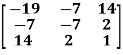
Sol. As we know that if the transpose of the given matrix is same as the matrix itself then the matrix is called symmetric matrix.
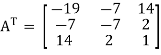
So that, first we will find its transpose,
Transpose of matrix A ,
Here,
A = 
The matrix A is symmetric.
Example: Show that any square matrix can be expressed as the sum of symmetric matrix and anti- symmetric matrix.
Solution. Suppose A is any square matrix.
Then,
A = 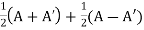
Now,
(A + A’)’ = A’ + A
A+A’ is a symmetric matrix.
Also,
(A - A’)’ = A’ – A
Here A’ – A is an anti – symmetric matrix
So that,
Square matrix = symmetric matrix + anti-symmetric matrix
Hermitian matrix:
A square matrix A =  is said to be hermitian matrix if every element of A is equal to conjugate complex j-ith element of A.
It means,

For example:
Necessary and sufficient condition for a matrix A to be hermitian –
A = (͞A)’
Skew-Hermitian matrix-
A square matrix A =  is said to be hermitian matrix if every element of A is equal to negative conjugate complex j-ith element of A.

Note- all the diagonal elements of a skew hermitian matrix are either zero or pure imaginary.
For example:
The necessary and sufficient condition for a matrix A to be skew hermitian will be as follows-
- A = (͞A)’
Note: A Hermitian matrix is a generalization of a real symmetric matrix and also every real symmetric matrix is Hermitian.
Similarly a Skew- Hermitian matrix is a generalization of a Skew symmetric matrix and also every Skew- symmetric matrix is Skew –Hermitian.
Theorem: Every square complex matrix can be uniquely expressed as sum hermitian and skew-hermitian matrix.
Or If A is given square complex matrix then  is hermitian and
  is skew-hermitian matrices.
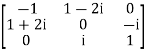
Example1: Express the matrix A as sum of hermitian and skew-hermitian matrix where 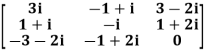
Let A =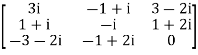
Therefore 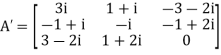 and
and 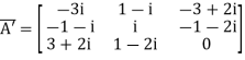
Let 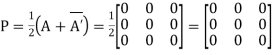
Again 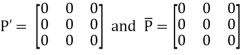
Hence P is a hermitian matrix.
Let 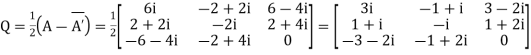
Again 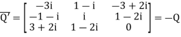
Hence Q is a skew- hermitian matrix.
We Check
P +Q=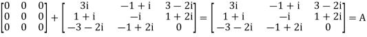
Hence proved.
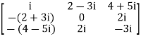
Example2: If A =  then show that
(i)  is hermitian matrix.
(ii)  is skew-hermitian matrix.
Sol.
Given A = 
Then 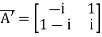
Let 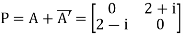
Also 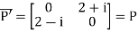
Hence P is a Hermitian matrix.
Let 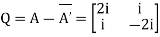
Also 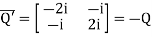
Hence Q is a skew-hermitian matrix.
Skew-symmetric matrix-
A square matrix A is said to be skew symmetrix matrix if –
1. A’ = -A, [ A’ is the transpose of A]
2.all the main diagonal elements will always be zero.
For example-
A = 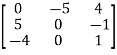
This is skew symmetric matrix, because transpose of matrix A is equals to negative A.
Example: check whether the following matrix A is symmetric or not?
A = 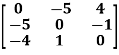
Solution This is not a skew symmetric matrix, because the transpose of matrix A is not equals to -A.
-A = A’
Orthogonal matrix-
Any square matrix A is said to be an orthogonal matrix if the product of the matrix A and its transpose is an identity matrix.
Such that,
A. A’ = I
Matrix × transpose of matrix = identity matrix
Note- if |A| = 1, then we can say that matrix A is proper.
Examples:  and
and 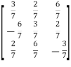 are the form of orthogonal matrices.
Unitary matrix-
A square matrix A is said to be unitary matrix if the product of the transpose of the conjugate of matrix A and matrix itself is an identity matrix.
Such that,
( ͞A)’. A = I
For example:

and its
Then (͞A)’ . A = I
So that we can say that matrix A is said to be a unitary matrix.
Key takeaways-
A = 
Where, i = 1, 2, …….,m and j = 1,2,3,…….n
Here ‘i’ denotes row and ‘j’ denotes column.
3. Any square matrix is said to be symmetric matrix if its transpose equals to the matrix itself.
4. Square matrix = symmetric matrix + anti-symmetric matri
5. A square matrix A =  is said to be hermitian matrix if every element of A is equal to conjugate complex j-ith element of A.
6. All the diagonal elements of a skew hermitian matrix are either zero or pure imaginary.
7. A Hermitian matrix is a generalization of a real symmetric matrix and also every real symmetric matrix is Hermitian
8. Every square complex matrix can be uniquely expressed as sum hermitian and skew-hermitian matrix.
9. A square matrix A is said to be skew symmetric matrix if –
(a) A’ = -A, [ A’ is the transpose of A]
(b) all the main diagonal elements will always be zero.
10. Any square matrix A is said to be an orthogonal matrix if the product of the matrix A and its transpose is an identity matrix.
11. if |A| = 1, then we can say that matrix A is proper.
12. A square matrix A is said to be unitary matrix if the product of the transpose of the conjugate of matrix A and matrix itself is an identity matrix.
Algebra on Matrices:
Addition and subtraction of matrices is possible if and only if they are of same order.
We add or subtract the corresponding elements of the matrices.
Example: 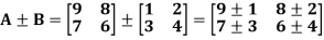
Example: Add 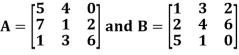 .
.
Sol.
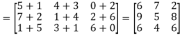
A + B = 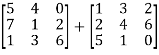
2. Scalar multiplication of matrix:
In this we multiply the scalar or constant with each element of the matrix.
Example: 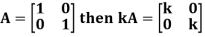
3. Multiplication of matrices: Two matrices can be multiplied only if they are conformal i.e. the number of column of first matrix is equal to the number rows of the second matrix.
Example: 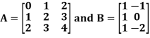
Then 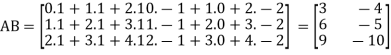
4. Power of Matrices: If A is A square matrix then

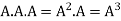 and so on.
If  where A is square matrix then it is said to be idempotent.
5. Transpose of a matrix: The matrix obtained from any given matrix A , by interchanging rows and columns is called the transpose of A and is denoted by 
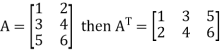
The transpose of matrix 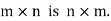 Also
Also 
Note: 
6. Trace of a matrix-
Suppose A be a square matrix, then the sum of its diagonal elements is known as trace of the matrix.
Example- If we have a matrix A-

Then the trace of A = 0 + 2 + 4 = 6
Key takeaways-


If A be a square matrix, then the sum of its diagonal elements is known as trace of the matrix
Determinants
The determinant of a square matrix is a number that associated with the square matrix. This number may be positive, negative or zero.
The determinant of the matrix A is denoted by det A or |A| or D
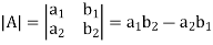
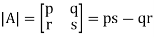
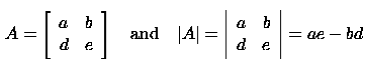
For 2 by 2 matrix-

Determinant will be
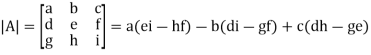
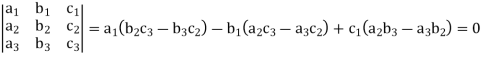
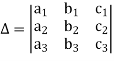
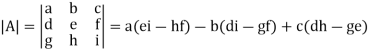
For 3 by 3 matrix-

Determinant will be
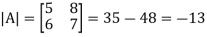
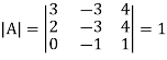
Example: If A =  then find |A|.
Sol.
As we know that-
Then-
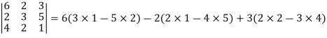
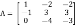
Example: Find out the determinant of the following matrix A.
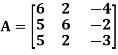
Solution
By the rule of determinants-
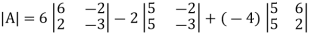


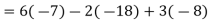
Example: expand the determinant:

Sol. As we know
Then,


Minor –
The minor of an element is define as determinant obtained by deleting the row and column containing the element.
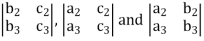
In a determinant,

The minor of  are given by

Cofactor –
Cofactors can be defined as follows,
Cofactor =  minor
minor
Where r is the number of rows and c is the number of columns.
Example: Find the minors and cofactors of the first row of the determinant.

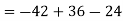
Sol. (1) The minor of element 2 will be,
Delete the corresponding row and column of element 2,
We get,
Which is equivalent to, 1 × 7 - 0 × 2 = 7 – 0 = 7
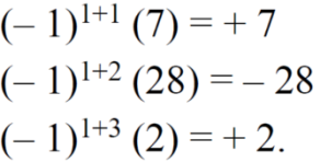
Similarly the minor of element 3 will be,
4× 7 - 0× 6 = 28 – 0 = 28
Minor of element 5,
4 × 2 - 1× 6 = 8 – 6 = 2
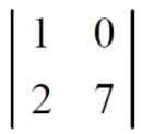
The cofactors of 2, 3 and 5 will be,
Properties of determinants-
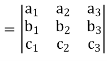
(1) If the rows are interchanged into columns or columns into rows then the value of determinants does not change.
Let us consider the following determinant:


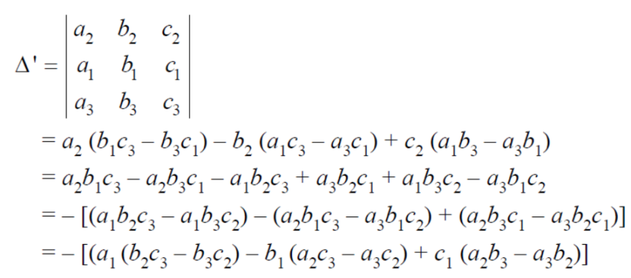
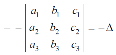
(2) The sign of the value of determinant changes when two rows or two columns are interchanged.
Interchange the first two rows of the following, we get
(3) If two rows or two columns are identical the the value of determinant will be zero.
Let, the determinant has first two identical rows,
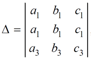
As we know that if we interchange the first two rows then the sign of the value of the determinant will be changed, so that

Hence proved
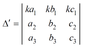
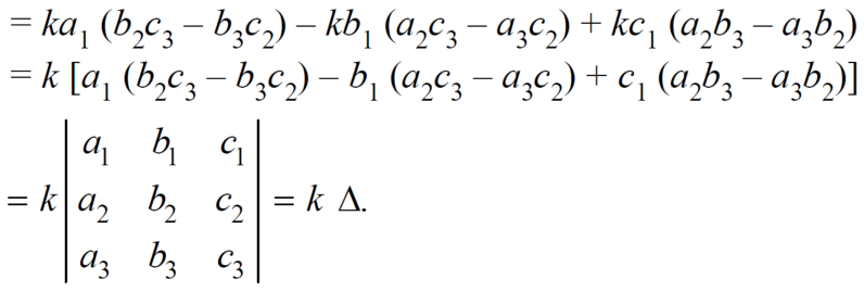
(4) if the element of any row of a determinant be each multiplied by the same number then the determinant multiplied by the same number,
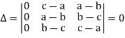
Example: Show that,
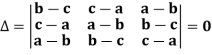
Solution Applying
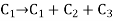
We get,
Example: Solve-
Sol:
Given
Apply- 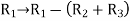
We get-
Applications of determinants-
Determinants have various applications such as finding the area and condition of collinearity.
Area of triangles-
Suppose the three vertices of a triangle are 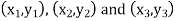 respectively, then we know that the area of the triangle is given by-
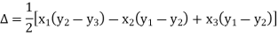
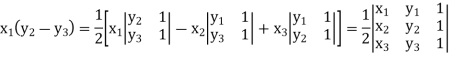
This is how we can find the area of the triangle.
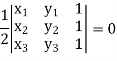
Condition of collinearity-
Let there are three points 
Then these three points will be collinear if -

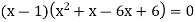
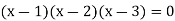
Example: Show that the points given below are collinear-
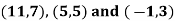
Solution
First we need to find the area of these points and if the area is zero then we can say that these are collinear points-
So that-
We know that area enclosed by three points-
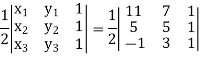
Apply- 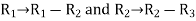
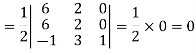
So that these points are collinear.
Key takeaways-
In a determinant,

The minor of  are given by
4. Cofactors can be defined as follows,
Cofactor =  minor
minor
Where r is the number of rows and c is the number of columns.
5. If the rows are interchanged into columns or columns into rows then the value of determinants does not change.
6. The sign of the value of determinant changes when two rows or two columns are interchanged.
7. If two rows or two columns are identical the the value of determinant will be zero.
8. if the element of any row of a determinant be each multiplied by the same number then the determinant multiplied by the same number
9. If the three vertices of a triangle are  respectively, then we know that the area of the triangle is given by-


10. Condition of collinearity-
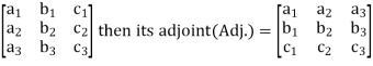
Adjoint of a matix-
Transpose of a co-factor matrix is known as the disjoint matrix.
If the following is a co-factor of matrix A-

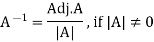
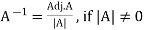
Inverse of a matrix-
The inverse of a matrix ‘A’ can be find as-
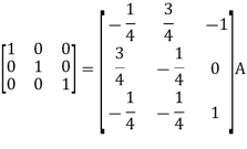
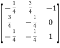
Example: Find the inverse of matrix ‘A’ if-
Solution
Here we have-
Then
And the matrix formed by its co-factors of |A| is-
Then

Therefore-
We know that-

Inverse of a matrix by using elementary transformation-
The following transformation are defined as elementary transformations-
1. Interchange of any two rows (column)
2. Multiplication of any row or column by any non-zero scalar quantity k.
3. Addition to one row (column) of another row(column) multiplied by any non-zero scalar.
The symbol ~ is used for equivalence.
Elementary matrices-
If we get a square matrix from an identity or unit matrix by using any single elementary transformation is called elementary matrix.
Note- Every elementary row transformation of a matrix can be affected by pre multiplication with the corresponding elementary matrix.
The method of finding inverse of a non-singular matrix by using elementary transformation-
Working steps-
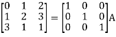
1. Write A = IA
2. Perform elementary row transformation of A of the left side and I on right side.
3. Apply elementary row transformation until ‘A’ (left side) reduces to I, then I reduces to 
Example-1: Find the inverse of matrix ‘A’ by using elementary transformation-
A = 
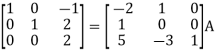
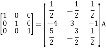
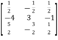
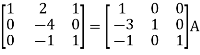
Solution Write the matrix ‘A’ as-
A = IA
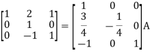
Apply  , we get
Apply 
Apply 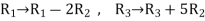
Apply 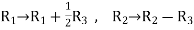
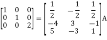
Apply 
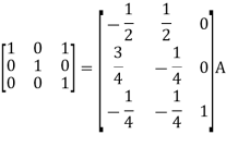
So that,
 =
= 
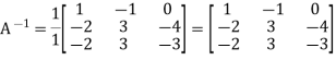
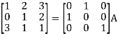
Example-2: Find the inverse of matrix ‘A’ by using elementary transformation-
A = 
Solution Write the matrix ‘A’ as-
A = IA
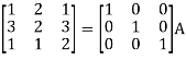
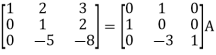
Apply 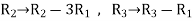
Apply 
Apply 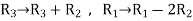
Apply 
So that
 =
= 
Key takeaways-
If the following is a co-factor of matrix A-
2. 
3. If we get a square matrix from an identity or unit matrix by using any single elementary transformation is called elementary matrix.
4. Every elementary row transformation of a matrix can be affected by pre multiplication with the corresponding elementary matrix.
5. The symbol ~ is used for equivalence.
Homogeneous System of Linear equations,
For a homogeneous system of equations ax+by=0 and cx+dy=0, the situation is slightly different. These lines pass through the origin. Thus, there is always at least one solution, the point (0,0). If the slopes -a/b and -c/d are equal then there are an infinite number of solutions since the lines are identical. But as we have seen, the slopes of these lines are equal when the determinant of the coefficient matrix is zero. Thus, for homogeneous systems we have the following result:
A nxn homogeneous system of linear equations has a unique solution (the trivial solution) if and only if its determinant is non-zero. If this determinant is zero, then the system has an infinite number of solutions.
A system of linear equations is homogeneous if all of the constant terms are zero:
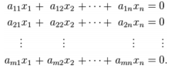
A homogeneous system is equivalent to a matrix equation of the form
Ax= 0
where A is an m × n matrix, x is a column vector with n entries, and 0 is the zero vector with m entries.
Example
Let 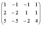 . Find the solution of the homogeneous system of linear equations
Ax = 0
Solution
Transform the coefficient matrix to the row echelon form:
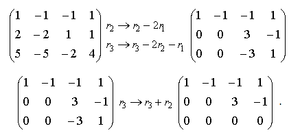
Since , we have to consider two unknowns as leading unknowns and to assign parametric values to the other unknowns. Setting x2=c1 and x3=c2 we obtain the following homogeneous linear system:
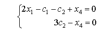
Therefore
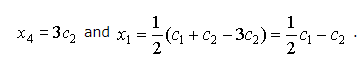
Thus, the given system has the following general solution:
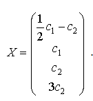
In view of the matrix properties, the general solution can be also expressed as the linear combination of particular solutions:
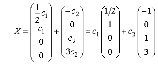
The particular solutions and form the fundamental system of solutions.
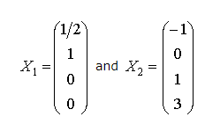
Thus,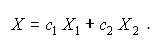
Condition for Consistency of homogeneous system,
A linear system is consistent if it has a solution, and inconsistent otherwise. When the system is inconsistent, it is possible to derive a contradiction from the equations, that may always be rewritten such as the statement 0 = 1.
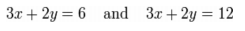
For example, the equations are inconsistent. In fact, by subtracting the first equation from the second one and multiplying both sides of the result by 1/6, we get 0 = 1. The graphs of these equations on the xy-plane are a pair of parallel lines.
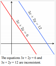
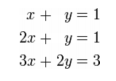
It is possible for three linear equations to be inconsistent, even though any two of them are consistent together. For example, the equations are inconsistent. Adding the first two equations together gives 3x + 2y = 2, which can be subtracted from the third equation to yield 0 = 1. Note that any two of these equations have a common solution. The same phenomenon can occur for any number of equations.
In general, inconsistencies occur if the left-hand sides of the equations in a system are linearly dependent, and the constant terms do not satisfy the dependence relation. A system of equations whose left-hand sides are linearly independent is always consistent.
Putting it another way, according to the Rouché–Capelli theorem, any system of equations (over determined or otherwise) is inconsistent if the rank of the augmented matrix is greater than the rank of the coefficient matrix. If, on the other hand, the ranks of these two matrices are equal, the system must have at least one solution. The solution is unique if and only if the rank equals the number of variables. Otherwise the general solution has k free parameters where k is the difference between the number of variables and the rank; hence in such a case there are an infinitude of solutions.
Solution of Non-homogeneous System of Linear equations (not more than three variables),
For square systems of equations (i.e. those with an equal number of equations and unknowns), the most powerful tool for determining the number of solutions the system has is the determinant. Suppose we have two equations and two unknowns: ax+by=c and dx+ey=f with b and e non-zero (i.e. the system is nonhomogeneous). These are two lines with slope -a/b and -d/e, respectively. Let's define the determinant of a 2x2 system of linear equations to be the determinant of the matrix of coefficients A of the system. For this system
Suppose this determinant is zero. Then, this last equation implies a/b=d/e; in other words, the slopes are equal. From our discussion above, this means the lines are either identical (there is an infinite number of solutions) or parallel (there are no solutions). If the determinant is non-zero, then the slopes must be different and the lines must intersect in exactly one point. This leads us to the following result:
A nxn nonhomogeneous system of linear equations has a unique non-trivial solution if and only if its determinant is non-zero. If this determinant is zero, then the system has either no nontrivial solutions or an infinite number of solutions.
Applications in Business and Economics,
Mathematics is used in almost every field of daily life. Business involves the buying and selling of goods in order to earn profit, it uses mathematics to record, classify, summarize and analyse the business transactions. So mathematics is used by commercial enterprises to record and manage the business operations such as, elementary arithmetic involving fractions, decimals, percentage, elementary algebra, statistics and probability. Now a days business management is using advanced mathematics such as calculus matrix algebra and liner programming. Practical applications include checking accounts, forecasting the sales, price discounts, mark-ups, mark-downs, payroll calculations, simple and compound interest, reducing wastage of resources.
Matrices play prominent role in developing a solution required for commercial organizations. It has knowledge to deal with unique needs of various sectors of Industry. It gives opportunities to finance and logistics management and customer relationship by providing them a variety of solutions. Also product price matrices are helpful to set bulk purchase discount. Determinants and Cramer rule are helpful in problem solving related to business and economy. It enables oneself in obtaining and optimal solution to maximize profit or minimize cost problems. Linear algebra serves a purpose of powerful tool for its application in business. As total cost, revenue, supply, demand and population are all related with a system of linear equations.
Quantitative methods are mathematical or statistical calculations that provide economists with indicators for comparing the current economic analysis to those of previous periods. Economists often use various types of math to ensure their personal judgments, inferences or theories are supported by meaningful calculations. Mathematical economics is the application of mathematical methods such as differential and integral calculus, difference and differential equations, matrix algebra, mathematical programming, and other computational methods to represent theories and analyze problems in economics
Examples and Problems
Example 1
Let. 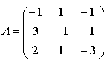 Solve the following homogeneous system of linear equations
Ax= 0
Explain why there are no solutions, an infinite number of solutions, or exactly one solution.
Solution
Note that any homogeneous system is consistent and has at least the trivial solution.
Transform the coefficient matrix to the triangular or row echelon form.
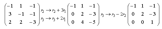
The rank of A equals 3. Therefore, there are no free variables and the system
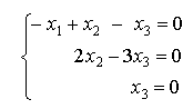
has only the trivial solution:
Example 2
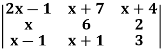
For what value of k doe the following homogeneous system of equations posses a non-trivial solution: x + ky + 3z = 0, kx + ky - 2z = 0, 2x + 3y - 4z = 0.
Solution
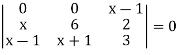
For non-trivial solution i.e. D = 0.
D =  = 0.
= 0.
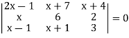
Apply R2 - 3R1 and R3 - 2R1 => 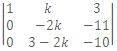 = 0.
= 0.
Expanding by 1st column, we get k = 33/2.
References-


