UNIT 3
Correlation and Regression
Correlation is used to describe the linear relationship between two continuous variables (e.g., height and weight). In general, correlation tends to be used when there is no identified response variable. It measures the strength (qualitatively) and direction of the linear relationship between two or more variables.
Definition
“Correlation analysis deals with the association between two or more variables.” —Simpson and Kafka
“Correlation is an analysis of the co-variation between two variables.” —A.M. Tuttle
Types
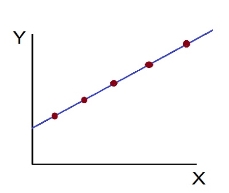
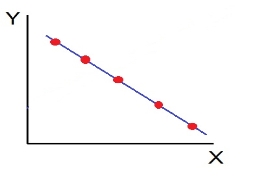
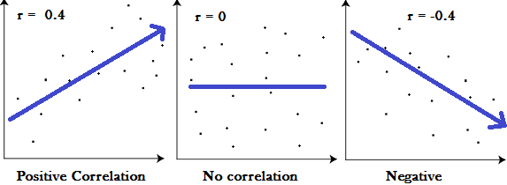
Correlation measures the nature and strength of relationship between two variables. Correlation lies between +1 to -1. A correlation of +1 indicates a perfect positive correlation between two variables. A zero correlation indicates that there is no relationship between the variables. A correlation of -1 indicates a perfect negative correlation.

Scatter diagram
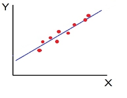
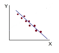
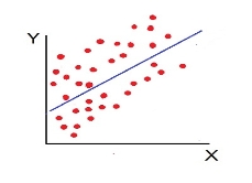
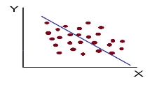
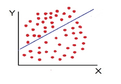
Scatter diagram method is the simplest method to study correlation between two variables. The correlations of two variables are plotted in the graph in the form of dots thereby obtaining as many points as the number of observations. The degree of correlation is ascertained by looking at the scattered points over the charts.
The more the points plotted are scattered over the chart, the lesser is the degree of correlation between the variables. The more the points plotted are closer to the line, the higher is the degree of correlation. The degree of correlation is denoted by “r”.
Interpretation with respect to magnitude and direction of relationship
Correlation coefficients index the extent to which two scores are related, and the direction of that relationship. They reflect the tendency of the variables to “co-vary”; that is, for changes in the value of one variable to be associated with changes in the value of the other. In interpreting correlation coefficients, two properties are important.
Key takeaways
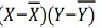
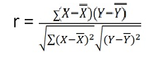
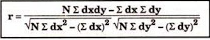
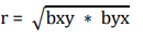
Karl Pearson’s Coefficient of Correlation is widely used mathematical method is used to calculate the degree and direction of the relationship between linear related variables. The coefficient of correlation is denoted by “r”.
Direct method
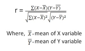
The value of the coefficient of correlation (r) always lies between ±1. Such as:
Example 1 - Compute Pearson’s coefficient of correlation between advertisement cost and sales as per the data given below:
Advertisement cost | 39 | 65 | 62 | 90 | 82 | 75 | 25 | 98 | 36 | 78 |
sales | 47 | 53 | 58 | 86 | 62 | 68 | 60 | 91 | 51 | 84 |
Solution
X | Y |
|
|
|
| |
39 | 47 | -26 | 676 | -19 | 361 | 494 |
65 | 53 | 0 | 0 | -13 | 169 | 0 |
62 | 58 | -3 | 9 | -8 | 64 | 24 |
90 | 86 | 25 | 625 | 20 | 400 | 500 |
82 | 62 | 17 | 289 | -4 | 16 | -68 |
75 | 68 | 10 | 100 | 2 | 4 | 20 |
25 | 60 | -40 | 1600 | -6 | 36 | 240 |
98 | 91 | 33 | 1089 | 25 | 625 | 825 |
36 | 51 | -29 | 841 | -15 | 225 | 435 |
78 | 84 | 13 | 169 | 18 | 324 | 234 |
650 | 660 |
| 5398 |
| 2224 | 2704 |
|
|
|
|
|
|
|


r = (2704)/√5398 √2224 = (2704)/(73.2*47.15) = 0.78
Thus Correlation coefficient is positively correlated
Example 2
Compute correlation coefficient from the following data
Hours of sleep (X) | Test scores (Y) |
8 | 81 |
8 | 80 |
6 | 75 |
5 | 65 |
7 | 91 |
6 | 80 |
X | Y |
|
|
|
| |
8 | 81 | 1.3 | 1.8 | 2.3 | 5.4 | 3.1 |
8 | 80 | 1.3 | 1.8 | 1.3 | 1.8 | 1.8 |
6 | 75 | -0.7 | 0.4 | -3.7 | 13.4 | 2.4 |
5 | 65 | -1.7 | 2.8 | -13.7 | 186.8 | 22.8 |
7 | 91 | 0.3 | 0.1 | 12.3 | 152.1 | 4.1 |
6 | 80 | -0.7 | 0.4 | 1.3 | 1.8 | -0.9 |
40 | 472 |
| 7 |
| 361 | 33 |


X = 40/6 =6.7

Y = 472/6 = 78.7

r = (33)/√7 √361 = (33)/(2.64*19) = 0.66
Thus Correlation coefficient is positively correlated
Example 3
Calculate coefficient of correlation between X and Y series using Karl Pearson shortcut method
X | 14 | 12 | 14 | 16 | 16 | 17 | 16 | 15 |
Y | 13 | 11 | 10 | 15 | 15 | 9 | 14 | 17 |
Solution
Let assumed mean for X = 15, assumed mean for Y = 14
X | Y | dx | dx2 | dy | dy2 | dxdy |
14 | 13 | -1.0 | 1.0 | -1.0 | 1.0 | 1.0 |
12 | 11 | -3.0 | 9.0 | -3.0 | 9.0 | 9.0 |
14 | 10 | -1.0 | 1.0 | -4.0 | 16.0 | 4.0 |
16 | 15 | 1.0 | 1.0 | 1.0 | 1.0 | 1.0 |
16 | 15 | 1.0 | 1.0 | 1.0 | 1.0 | 1.0 |
17 | 9 | 2.0 | 4.0 | -5.0 | 25.0 | -10.0 |
16 | 14 | 1 | 1 | 0 | 0 | 0 |
15 | 17 | 0 | 0 | 3 | 9 | 0 |
120 | 104 | 0 | 18 | -8 | 62 | 6 |

 r = 8 *6 – (0)*(-8)
√8*18-(0)2 √8*62 – (-8)2
r = 48/√144*√432 = 0.19
Example 4 - Calculate coefficient of correlation between X and Y series using Karl Pearson shortcut method
X | 1800 | 1900 | 2000 | 2100 | 2200 | 2300 | 2400 | 2500 | 2600 |
F | 5 | 5 | 6 | 9 | 7 | 8 | 6 | 8 | 9 |
Solution
Assumed mean of X and Y is 2200, 6
X | Y | dx | dx (i=100) | dx2 | dy | dy2 | dxdy |
1800 | 5 | -400 | -4 | 16 | -1.0 | 1.0 | 4.0 |
1900 | 5 | -300 | -3 | 9 | -1.0 | 1.0 | 3.0 |
2000 | 6 | -200 | -2 | 4 | 0.0 | 0.0 | 0.0 |
2100 | 9 | -100 | -1 | 1 | 3.0 | 9.0 | -3.0 |
2200 | 7 | 0 | 0 | 0 | 1.0 | 1.0 | 0.0 |
2300 | 8 | 100 | 1 | 1 | 2.0 | 4.0 | 2.0 |
2400 | 6 | 200 | 2 | 4 | 0 | 0 | 0.0 |
2500 | 8 | 300 | 3 | 9 | 2 | 4 | 6.0 |
2600 | 9 | 400 | 4 | 16 | 3 | 9 | 12.0 |
|
|
|
|
|
|
|
|
|
|
| 0 | 60 | 9 | 29 | 24 |
Note – we can also proceed dividing x/100
 r = (9)(24) – (0)(9)
√9*60-(0)2 √9*29– (9)2
r = 0.69
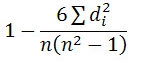
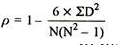
Key Takeaways:
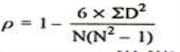
Where, P = Rank coefficient of correlation
D = Difference of ranks
N = Number of Observations
The Spearman’s Rank Correlation coefficient lies between +1 to -1.
When ranks are not given - Rank by taking the highest value or the lowest value as 1
Equal Ranks or Tie in Ranks – in this case ranks are assigned on an average basis. For ex – if three students score of 5, at 5th, 6th, 7th ranks ach one of them will be assigned a rank of 5 + 6 + 7/3= 6.
If two individual ranked equal at third position, then the rank is calculates as (3+4)/2 = 3.5
Example 1 –
Test 1 | 8 | 7 | 9 | 5 | 1 |
Test 2 | 10 | 8 | 7 | 4 | 5 |
Solution
Here, highest value is taken as 1
Test 1 | Test 2 | Rank T1 | Rank T2 | D | d2 |
8 | 10 | 2 | 1 | 1 | 1 |
7 | 8 | 3 | 2 | 1 | 1 |
9 | 7 | 1 | 3 | -2 | 4 |
5 | 4 | 4 | 5 | -1 | 1 |
1 | 5 | 5 | 4 | 1 | 1 |
|
|
|
|
| 8 |

R = 1 – (6*8)/5(52 – 1) = 0.60
Example 2 -
Calculate Spearman rank-order correlation
English | 56 | 75 | 45 | 71 | 62 | 64 | 58 | 80 | 76 | 61 |
Maths | 66 | 70 | 40 | 60 | 65 | 56 | 59 | 77 | 67 | 63 |
Solution
Rank by taking the highest value or the lowest value as 1.
Here, highest value is taken as 1
English | Maths | Rank (English) | Rank (Math) | d | d2 |
56 | 66 | 9 | 4 | 5 | 25 |
75 | 70 | 3 | 2 | 1 | 1 |
45 | 40 | 10 | 10 | 0 | 0 |
71 | 60 | 4 | 7 | -3 | 9 |
62 | 65 | 6 | 5 | 1 | 1 |
64 | 56 | 5 | 9 | -4 | 16 |
58 | 59 | 8 | 8 | 0 | 0 |
80 | 77 | 1 | 1 | 0 | 0 |
76 | 67 | 2 | 3 | -1 | 1 |
61 | 63 | 7 | 6 | 1 | 1 |
|
|
|
|
| 54 |

 R = 1-(6*54)
10(102-1)
R = 0.67
Therefore this indicates a strong positive relationship between the ranks individuals obtained in the math and English exam.
Example 3 –
Find Spearman's rank correlation coefficient between X and Y for this set of data:
X | 13 | 20 | 22 | 18 | 19 | 11 | 10 | 15 |
Y | 17 | 19 | 23 | 16 | 20 | 10 | 11 | 18 |
Solution
X | Y | Rank X | Rank Y | D | d2 |
13 | 17 | 3 | 4 | -1 | 1 |
20 | 19 | 7 | 6 | 1 | 1 |
22 | 23 | 8 | 8 | 0 | 0 |
18 | 16 | 5 | 3 | 2 | 2 |
19 | 20 | 6 | 7 | -1 | 1 |
11 | 10 | 2 | 1 | 1 | 1 |
10 | 11 | 1 | 2 | -1 | 1 |
15 | 18 | 4 | 5 | -1 | 1 |
|
|
|
|
| 8 |
R =

 R = 1 – 6*8/8(82 – 1) = 1 – 48 = 0.90
504
Example 4 – calculation of equal ranks or tie ranks
Find Spearman's rank correlation coefficient:
Commerce | 15 | 20 | 28 | 12 | 40 | 60 | 20 | 80 |
Science | 40 | 30 | 50 | 30 | 20 | 10 | 30 | 60 |
Solution
C | S | Rank C | Rank S | D | d2 |
15 | 40 | 2 | 6 | -4 | 16 |
20 | 30 | 3.5 | 4 | -0.5 | 0.25 |
28 | 50 | 5 | 7 | -2 | 4 |
12 | 30 | 1 | 4 | -3 | 9 |
40 | 20 | 6 | 2 | 4 | 16 |
60 | 10 | 7 | 1 | 6 | 36 |
20 | 30 | 3.5 | 4 | -0.5 | 0.25 |
80 | 60 | 8 | 8 | 0 | 0 |
|
|
|
|
| 81.5 |

R = 1 – (6*81.5)/8(82 – 1) = 0.02
Key takeaways - The Spearman’s Rank Correlation Coefficient is the non-parametric statistical measure used to study the strength of association between the two ranked variables.
Concept
Regression analysis is a technique of studying the dependence of one variable called dependent variable, on one or more variable called explanatory variable, with a view to estimate or predict the average value of the dependent variables in terms of the known or fixed values of the independent variables.
Regression analysis includes several variations, such as linear, multiple linear, and nonlinear. The most common models are simple linear and multiple linear.
Nonlinear regression analysis is commonly used for more complicated data sets in which the dependent and independent variables show a nonlinear relationship.
Linear model assumption
Lines for regression for ungrouped data
Simple linear regression
Simple linear regression is a model that assesses the relationship between a dependent variable and an independent variable.
Y = a + bX + ϵ
Where:
Y – Dependent variable
X – Independent (explanatory) variable
a – Intercept
b – Slope
ϵ – Residual (error)
With the help of simple linear regression model we have the following two regression lines
1. Regression line of Y on X: This line gives the probable value of Y (Dependent variable) for any given value of X (Independent variable).
Regression line of Y on X : Y – Ẏ = byx (X – Ẋ)
OR : Y = a + bX
2. Regression line of X on Y: This line gives the probable value of X (Dependent variable) for any given value of Y (Independent variable).
Regression line of X on Y : X – Ẋ = bxy (Y – Ẏ)
OR : X = a + bY
Multiple linear regressions
Multiple linear regression analysis is essentially similar to the simple linear model, with the exception that multiple independent variables are used in the model.
Y = a + bX1 + cX2 + dX3 + ϵ
Where:
Y – Dependent variable
X1, X2, X3 – Independent (explanatory) variables
a – Intercept
b, c, d – Slopes
ϵ – Residual (error)

Example
How to find a linear regression equation
Subject | X | Y |
1 | 43 | 99 |
2 | 21 | 65 |
3 | 25 | 79 |
4 | 42 | 75 |
5 | 57 | 87 |
6 | 59 | 81 |
|
|
|
Solution
Subject | X | Y | Xy | X2 | Y2 |
1 | 43 | 99 | 4257 | 1849 | 9801 |
2 | 21 | 65 | 1365 | 441 | 4225 |
3 | 25 | 79 | 1975 | 625 | 6241 |
4 | 42 | 75 | 3150 | 1764 | 5625 |
5 | 57 | 87 | 4959 | 3249 | 7569 |
6 | 59 | 81 | 4779 | 3481 | 6521 |
Total | 247 | 486 | 20485 | 11409 | 40022 |
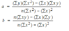
To find a and b, use the following equation
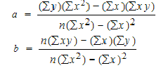
Find a:
((486 × 11,409) – ((247 × 20,485)) / 6 (11,409) – 247*247)
484979 / 7445
=65.14
Find b:
(6(20,485) – (247 × 486)) / (6 (11409) – 247*247)
(122,910 – 120,042) / 68,454 – 2472
2,868 / 7,445
= .385225
y’ = a + bx
y’ = 65.14 + .385225x
Example
Calculate linear regression analysis
students | X | Y |
1 | 95 | 85 |
2 | 85 | 95 |
3 | 80 | 70 |
4 | 70 | 65 |
5 | 60 | 70 |
Solution
students | X | Y | X2 | y2 | xy |
1 | 95 | 85 | 9025 | 7225 | 8075 |
2 | 85 | 95 | 7225 | 9025 | 8075 |
3 | 80 | 70 | 6400 | 4900 | 5600 |
4 | 70 | 65 | 4900 | 4225 | 4550 |
5 | 60 | 70 | 3600 | 4900 | 4200 |
total | 390 | 385 | 31150 | 30275 | 30500 |
To find a and b, use the following equation
Find a:
((385 × 31150) – ((390 × 30500)) / 5 (31150) – 152100)
97750 / 3650
=26.78
Find b:
(5(30500) – (390 × 385)) / (5 (31150) – 152100)
2,350 / 3650
= .0.64
y’ = a + bx
y’ = 26.78 + .0.64x
Prediction using lines of regression
Regression analysis is a predictive modeling technique that estimates the relationship between two or more variables. Recall that a correlation analysis makes no assumption about the causal relationship between two variables. Regression analysis focuses on the relationship between a dependent (target) variable and an independent variable(s) (predictors). Here, the dependent variable is assumed to be the effect of the independent variable(s). The value of predictors is used to estimate or predict the likely-value of the target variable.
Key takeaways - Regression analysis includes several variations, such as linear, multiple linear, and nonlinear
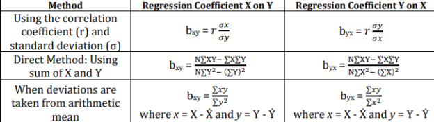
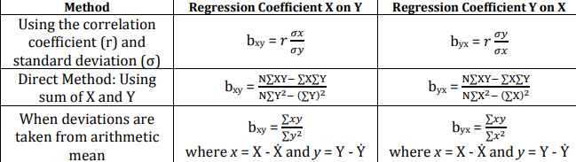
The quantity “b” in the regression equation is called as the regression coefficient or slope coefficient. Since there are two regression equations, therefore, we have two regression coefficients.
1. Regression Coefficient X on Y, symbolically written as “bxy”
2. Regression Coefficient Y on X, symbolically written as “byx”
Different formula’s used to compute regression coefficients:
Properties of Regression Coefficients:

Examples
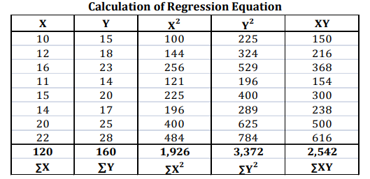
Find the two regression equation of X on Y and Y on X from the following data:
X: 10 12 16 11 15 14 20 22
Y: 15 18 23 14 20 17 25 28
Solution
Here N = Number of elements in either series X or series Y = 8
Now we will proceed to compute regression equations using normal equations.
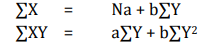
Regression equation of X on Y: X = a + bY
The two normal equations are:
Substituting the values in above normal equations, we get
120 = 8a + 160b ..... (i)
2542 = 160a + 3372b ..... (ii)
Let us solve these equations (i) and (ii) by simultaneous equation method
Multiply equation (i) by 20 we get 2400 = 160a + 3200b
Now rewriting these equations:
2400 = 160a + 3200b
2542 = 160a + 3372b
(-) (-) (-) .
-142 = -172b
Therefore now we have -142 = -172b, this can rewritten as 172b = 142
Now, b = 142/172 = 0.8256 (rounded off)
Substituting the value of b in equation (i), we get
120 = 8a + (160 * 0.8256)
120 = 8a + 132 (rounded off)
8a = 120 - 132
8a = -12
a = -12/8
a = -1.5
Thus we got the values of a = -1.5 and b = 0.8256
Hence the required regression equation of X on Y:
X = a + bY => X = -1.5 + 0.8256Y
Regression equation of Y on X: Y = a + bX
The two normal equations are:
∑Y = Na + b∑X
∑XY = a∑X + b∑X2
Substituting the values in above normal equations, we get
160 = 8a + 120b ..... (iii)
2542 = 120a + 1926b ..... (iv)
Let us solve these equations (iii) and (iv) by simultaneous equation method
Multiply equation (iii) by 15 we get 2400 = 120a + 1800b
Now rewriting these equations:
2400 = 120a + 1800b
2542 = 120a + 1926b
(-) (-) (-) .
-142 = -126b
Therefore now we have -142 = -126b, this can rewritten as 126b = 142
Now, b = 142/126 = 1.127 (rounded off)
Substituting the value of b in equation (iii), we get
160 = 8a + (120 * 1.127)
160 = 8a + 135.24
8a = 160 - 135.24
8a = 24.76
a = 24.76/8
a = 3.095
Thus we got the values of a = 3.095 and b = 1.127
Hence the required regression equation of Y on X:
Y = a + bX => Y = 3.095 + 1.127X
key takeaways - The quantity “b” in the regression equation is called as the regression coefficient or slope coefficient
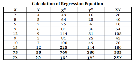
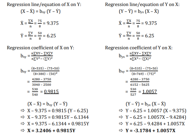
Examples and problems
Capital Employed (Rs. in lakh): 7 8 5 9 12 9 10 15
Sales Volume (Rs. in lakh): 4 5 2 6 9 5 7 12
Solution

2. After investigation it has been found the demand for automobiles in a city depends mainly, if not entirely, upon the number of families residing in that city. Below are the given figures for the sales of automobiles in the five cities for the year 2019 and the number of families residing in those cities.
Fit a linear regression equation of Y on X by the least square method and estimate the sales for the year 2020 for the city Belagavi which is estimated to have 100 lakh families assuming that the same relationship holds true.
Solution

Regression equation of Y on X: Y = a + bX
The two normal equations are:
∑Y = Na + b∑X
∑XY = a∑X + b∑X2
Substituting the values in above normal equations, we get
141.7 = 5a + 375b ..... (i)
10849= 375a + 28625b ..... (ii)
Let us solve these equations (i) and (ii) by simultaneous equation method
Multiply equation (i) by 75 we get 10627.5 = 375a + 28125b
Now rewriting these equations:
10627.5 = 375a + 28125b
10849 = 375a + 28625b
(-) (-) (-) .
-221.5 = -500b
Therefore now we have -221.5 = -500b, this can rewritten as 500b = 221.5
Now, b = 221.5/500 = 0.443
Substituting the value of b in equation (i), we get
141.7 = 5a + (375 * 0.443)
141.7 = 5a + 166.125
5a = 141.7 - 166.125
5a = -24.425
a = -24.425/5
a = -4.885
Thus we got the values of a = -4.885 and b = 0.443
Hence, the required regression equation of Y on X:
Y = a + bX => Y = -4.885 + 0.443X
Estimated sales of automobiles (Y) in city Belagavi for the year 2020, where number of families (X) are 100(in lakhs):
Y = -4.885 + 0.443X
Y = -4.885 + (0.443 * 100)
Y = -4.885 + 44.3
Y = 39.415 (‘000)
Means sales of automobiles would be 39,415 when number of families are 100,00,000
Example Given below are five observation collected in simple regression. Calculate the intercept, slope and write down the estimated regression equation
X | Y |
2 | 7 |
4 | 5 |
6 | 4 |
8 | 2 |
10 | 1 |
Solution
X | Y | X2 | y2 | xy |
2 | 7 | 4 | 49 | 14 |
4 | 5 | 16 | 25 | 20 |
6 | 4 | 36 | 16 | 24 |
8 | 2 | 64 | 4 | 16 |
10 | 1 | 100 | 1 | 10 |
30 | 19 | 220 | 95 | 84 |
To find a and b, use the following equation
Find a:
((19 × 220) – ((30 × 84)) / 5 (220) – 900)
1660/ 200
=8.3
Find b:
(5(84) – (30 × 19)) / (5 (220) – 900)
-150 / 200
= -0.75
y’ = a + bx
y’ = 8.3 + (-0.75)x
Example Calculate Karl Pearson’s Coefficient of Correlation
X | 28 | 45 | 40 | 38 | 35 | 33 | 40 | 32 | 36 | 33 |
Y | 23 | 34 | 33 | 34 | 30 | 26 | 28 | 31 | 36 | 35 |
Solution
X | Y |
|
|
|
| |
28 | 23 | -8 | 64 | -8.0 | 64.0 | 64.0 |
45 | 34 | 9 | 81 | 3.0 | 9.0 | 27.0 |
40 | 33 | 4 | 16 | 2.0 | 4.0 | 8.0 |
38 | 34 | 2 | 4 | 3.0 | 9.0 | 6.0 |
35 | 30 | -1 | 1 | -1.0 | 1.0 | 1.0 |
33 | 26 | -3 | 9 | -5.0 | 25.0 | 15.0 |
40 | 28 | 4 | 16 | -3 | 9 | -12.0 |
32 | 31 | -4 | 16 | 0 | 0 | 0.0 |
36 | 36 | 0 | 0 | 5 | 25 | 0.0 |
33 | 35 | -3 | 9 | 4 | 16 | -12 |
360 | 310 | 0 | 216 | 0 | 162 | 97 |


 X = 360/10 = 36
Y = 310/10 = 31

r = 97/(√216 √162 = 0.51
Example Calculates spearman rank correlation
X | 10 | 15 | 11 | 14 | 16 | 20 | 10 | 8 | 7 | 9 |
Y | 16 | 16 | 24 | 18 | 22 | 24 | 14 | 10 | 12 | 14 |
Solution
X | Y | Rank X | Rank Y | D | d2 |
10 | 16 | 6.5 | 5.5 | 1 | 1 |
15 | 16 | 3 | 5.5 | -2.5 | 6.25 |
11 | 24 | 5 | 1.5 | 3.5 | 12.25 |
14 | 18 | 4 | 4 | 0 | 0 |
16 | 22 | 2 | 3 | -1 | 1 |
20 | 24 | 1 | 1.5 | -0.5 | 0.25 |
10 | 14 | 6.5 | 7.5 | -1 | 1 |
8 | 10 | 9 | 10 | -1 | 1 |
7 | 12 | 10 | 9 | 1 | 1 |
9 | 14 | 8 | 7.5 | 0.5 | 0.25 |
|
|
|
|
| 24 |
R = 1 – (6*24)/10(102 – 1) = 0.85
The correlation between X and Y is positive and very high.
Example Find Karl Pearson’s coefficient of correlation between capital employed and profit obtained from the following data.
Solution
Let us assume that capital employed is variable X and profit is variable Y.
Example Find the correlation coefficient between age and playing habits of the following students using Karl Pearson’s coefficient of correlation method
Solution
To find the correlation between age and playing habits of the students, we need to compute the percentages of students who are having the playing habit.
Percentage of playing habits = No. of Regular Players / Total No. of Students * 100
Now, let us assume that ages of the students are variable X and percentages of playing habits are variable Y.
Interpretation: From the above calculation it is very clear that there is high degree of negative correlation i.e. r = -0.9912, between the two variables of age and playing habits. i.e. Playing habits among students decreases when their age increases.
Example Find out spearman’s coefficient of correlation between the two kinds of assessment of graduate students’ performance in a college.
Solution
Interpretation: From the above calculation it is very clear that there is high degree of positive correlation i.e. R = 0.7833, between two exams. It means there is a high degree of positive correlation between the internal exam and external exam of the students.
References-


