Unit 4
Measures of Central Tendency and Measures of Dispersion
After data collection, you may face the problem of arranging them into a format from which you will be able to draw some conclusions. The arrangement of these data in different groups on the basis of some similarities is known as classification. According to Tuttle, “ A classification is a scheme for breaking a category into a set of parts, called classes, according to some precisely defined differing characteristics possessed by all the elements of the category” Thus classification, is the process of grouping data into sequences according to their common characteristics, which separate them into different but related parts.
Such classification facilitates analysis of the data and consequently prepares a foundation for absolute interpretation of the obtained scores. The prime objective of the classification of data is concerned with reducing complexities with raw scores by grouping them into some classes. This will provides a comprehensive insight into the data.
The classification procedure in statistics enables the investigators to manage the raw scores in such a way that they can proceed with ease in a systematic and scientific manner.
Key takeaways –
- Raw data are classified in such a way its easy to understand through statistical methods
Both variable and attribute data measure the state of an object or a process, but the kind of information that each describes differs. Variable data involve numbers measured on a continuous scale, while attribute data involve characteristics or other information that you we quantify. Each has its own benefits over the others. Attributes are closely related to variables.
Example – age is an attribute that can be operationalised in many ways. It can represent two values old and young. In this case the attribute age is operationalised as a binary variable. If more than two values are possible and they can be ordered, the attribute is represented by ordinal variable such as young, middle and old.
Benefits
- Variable data provide detailed and concrete information about a product.
- Attribute data are often more helpful when qualitative information is needed.
Key takeaways –
- Variable means the measured values can vary anywhere along a given scale. Attribute data, on the other hand, is qualitative data that have a quality characteristic or attribute that is described in terms of measurements.
Classification of data is the process of arranging the data into homogenous groups according to their common characteristics. Raw data cannot be easily understood and not fit for analysis and interpretation. Therefore, arrangement of data helps the user in comparison and analysis.
Example- population of a state can be grouped according to sex, age, etc
Definition
“Classification is the process of arranging data into sequences according to their common characteristics or separating them into different related parts.” - Prof. Secrist
Objectives of data classification
- To consolidate the huge data in such a way that similarities and differences are easily understood.
- It helps in comparison and analysis of data
- Classification of data ensures prominent data are collected and optional data are separated
- To allow a statistical method of the material gathered.
- To study relationships
Types of classification
- Geographical classification – when the data classified according to the geographical location or regions (like states, cities, regions, zones, areas, etc). It is called geographical classification. It is also known as a real or spatial classification.
Ex- production of food grains are classified in different states in India
S.No | Name of states | Total food grains (000’ tones) |
1 | Andhra Pradesh | 1093.00 |
2 | Bihar | 12899.09 |
3 | Karnataka | 1834.70 |
4 | Punjab | 41289.00 |
5 | Orissa | 3600 |
2. Chronological classification – classification of data on the basis of time (like months, years, etc) of their occurrence are called chronological classification. This type of classification is suitable for data which takes place in course of time such as population, production, sales, etc.
Ex – profit of a company from 2001 to 2005
S.No | Year | Profits (in 000 Rs) |
1 | 2001 | 77 |
2 | 2002 | 88 |
3 | 2003 | 89 |
4 | 2004 | 94 |
5 | 2005 | 99 |
3. Qualitative classification – under this classification, the data are classified on the basis of some attributes or quality such as sex, color, literacy, honesty, intelligence, religion, etc. In this the attributes cannot be measured. This sort of classification is known as descriptive classification.
For example, Population can be divided on the basis of marital status as married or unmarried etc.
4. Quantitative classification – quantitative classification states that classification of data according to some characteristics that can be measured such as height, weight, income, sales, profit, etc.
Ex – students are classified according to weights
S.No | Weight | No. of students |
1 | 30-40 | 77 |
2 | 40-50 | 60 |
3 | 50-60 | 50 |
4 | 60 – 70 | 20 |
5. Alphabetical classification – when data are arranged according to alphabetical order is called alphabetical classification
Ex – state wise classification of population in alphabetical order
S.No | Name of states | Population |
1 | Andhra Pradesh | 157 |
2 | Bihar | 150 |
3 | Karnataka | 200 |
4 | Punjab | 700 |
5 | Orissa | 450 |
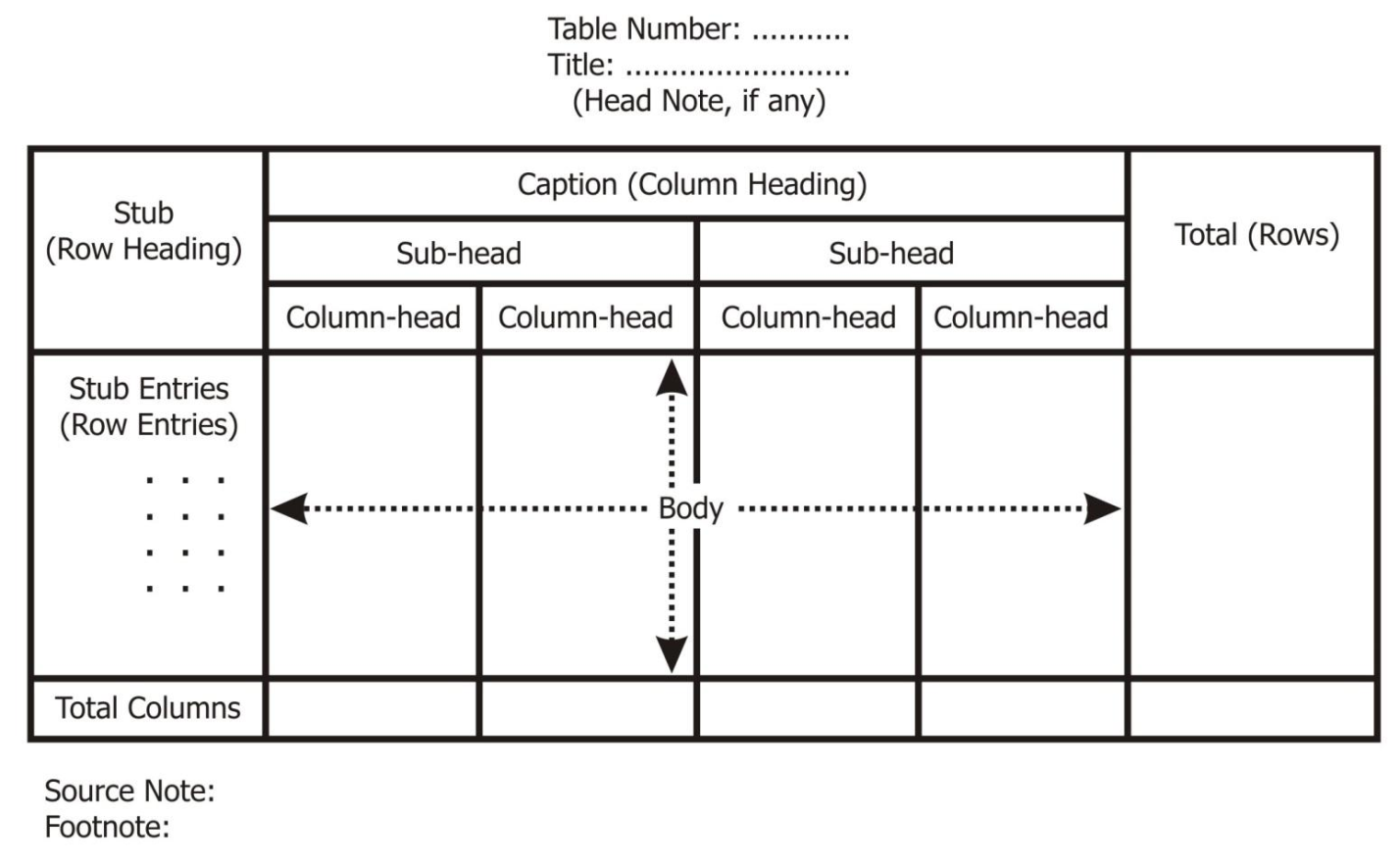
Tabulation is a systematic & logical presentation of numeric data in rows and columns, to facilitate comparison and statistical analysis. The method of placing organized data in tabular form is known as tabulation. Tabulation simplifies complex data and facilitates comparison.
Definition
“Table involves the orderly and systematic presentation of numerical data in a form designed to elucidate the problem under consideration” – According prof. L.R Connor
“Table in its broadest sense is an orderly arrangement of data in column and rows” – According to Prof M.M.Blaire
Objectives of tabulation
- It simplifies the raw data in meaningful form so that common man can easily understand in less time
- It brings essential facts in clear and precise manner
- Data presented in rows and columns helps in detailed comparison
- Tables serve as the best source of organized data for further statistical analysis
- Table saves the space without sacrificing the quality and quantity of data.
Parts of table
Table number |
|
Title of the table |
|
Caption |
|
Stub |
|
Body |
|
Head note |
|
Source note |
|
Footnote |
|
|
Types of tabulation
|
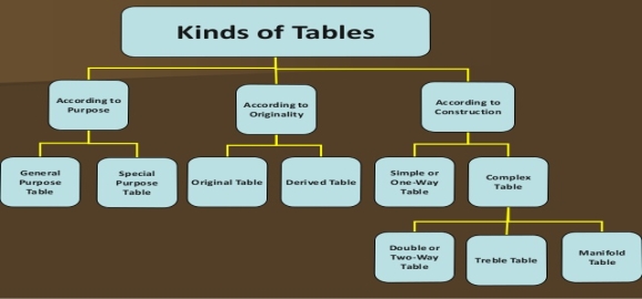
- According to purpose
- General purpose table – general purpose table is a table which is of general use. It does not serve any specific purpose under consideration
- Special purpose table – special purpose table is prepared with some specific purpose in mind.
2. According to originality
- Original table – an original table is that table in which data are presented in the same manner in which they are collected.
- Derived table – a derived table is that in which data is not presented in same manner in which they are collected. Here the data are first converted into ratio or percentage and then presented.
3. According to construction
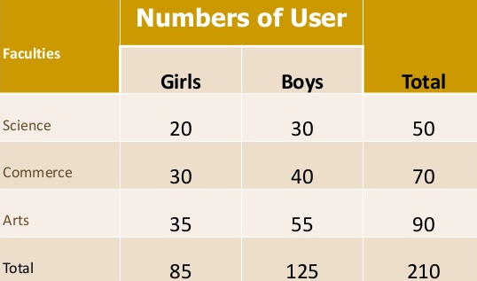
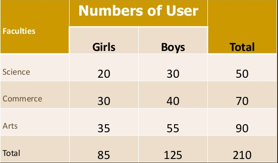
- Simple table – simple table also known as one-way table. Under this data are presented based on one characteristic
Faculty wise library user
|
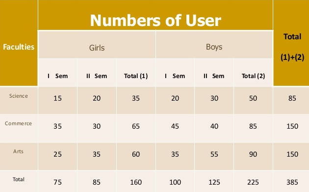
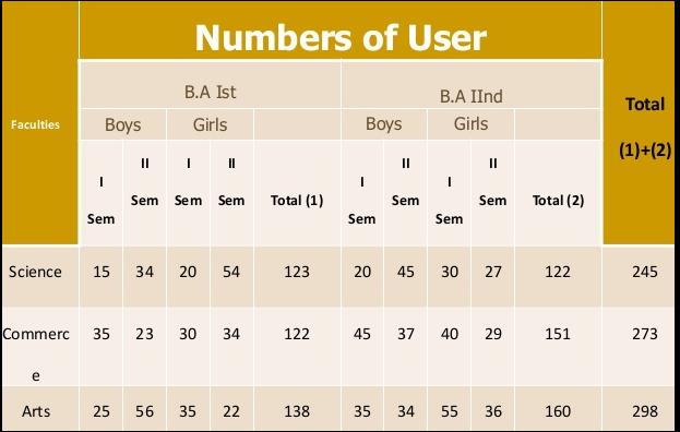
b. Complex tables – in complex table data are presented according to two or more characteristics simultaneously.
The complex tables are
- two way,
- three-way table and
- manifold table
Two-way table – Under this the variable under study is divided into two characteristics
|
Three-way table - Under this the variable under study is divided into three characteristics
|
Manifold table - Under this the variable under study is divided into large number of characteristics.
|
Key Takeaways:
- Table in its broadest sense is an orderly arrangement of data in column and rows.
- It simplifies the raw data in meaningful form so that common man can easily understand in less time.
Cumulative frequency is used to determine the number of observations that lie above (or below) a particular value in a data set. The cumulative frequency is calculated using a frequency distribution table, which can be constructed from stem and leaf plots or directly from the data.
The cumulative frequency is calculated by adding each frequency from a frequency distribution table to the sum of its predecessors. The last value will always be equal to the total for all observations, since all frequencies will already have been added to the previous total.
Histogram – histogram is a bar graph representing the frequency of occurrence by classes of data. In histogram data are plotted as a series of rectangle. ‘X axis’ consist of class intervals and ‘Y axis’ shows the frequencies. It is also called stair case or block diagram. Histogram is not suitable for open ended classes.
Ogive – An ogive graph shows cumulative frequency in statistics. It estimates the number of observations less than a given value or more than a given value. Cumulative frequency is obtained by adding to the given value
|
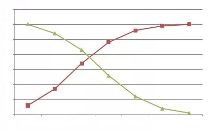
'Less than and equal to ogive: This consists of plotting the 'less than ' cumulative frequencies against the upper class boundaries of the respective classes. The points so obtained are joined by a smooth free hand curve to give 'less than ' ogive . Obviously, 'less than ' ogive is an increasing curve , sloping upwards from left to right .
‘More than and equal to’ ogive: This consists of plotting the ' more than ' cum. frequencies against the lower class boundaries of the respective classes . The points so obtained are joined by a smooth free hand curve to give ' equal give . Obviously, 'more than ' ogive is a decreasing curve , slopes downwards from left to right .
Key takeaways –
- The cumulative frequency is calculated by adding each frequency from a frequency distribution table to the sum of its predecessors.
- An ogive graph shows cumulative frequency in statistics
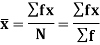
A measure of central tendency is a statistical summary that represents the center point of the dataset. It indicates where most values in a distribution fall. It is also called as measure of central location.
The three most common measure of central tendency are Mean, Median, and Mode.
Definition
According to Prof Bowley “Measures of central tendency (averages) are statistical constants which enable us to comprehend in a single effort the significance of the whole.”
Requisites of ideal measures of central tendency are as follows
- It should be rigidly defined
- It should be simple to understand and easy to calculate
- It should be based upon all values of given data.
- It should be capable of further mathematical treatment.
- It should have sampling stability.
- It should be not be unduly affected by extreme values.
Arithmetic mean
- The mean is the arithmetic average, also called as arithmetic mean.
- Mean is very simple to calculate and is most commonly used measure of the center of data.
- Means is calculated by adding up all the values and divided by the number of observations.
Merits of Mean
1)Arithmetic mean rigidly defined by Algebraic Formula.
2) It is easy to calculate and simple to understand.
3) It is based on all observations of the given data.
4) It is capable of being treated mathematically hence it is widely used in statistical analysis.
5) Arithmetic mean can be computed even if the derailed distribution is not known but some of the observation and number of the observation are known.
6) It is least affected by the fluctuation of sampling.
7) For every kind of data mean can be calculated.
Demerits of Arithmetic mean:
1) It can neither be determined by inspection or by graphical location.
2) Arithmetic mean cannot be computed for qualitative data like data on intelligence honesty and smoking habit etc.
3) It is too much affected by extreme observations and hence it is not adequately represent data consisting of some extreme point.
4) Arithmetic mean cannot be computed when class intervals have open ends.
5) If any one of the data is missing then mean cannot be calculated.
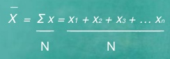
Computation of sample mean -
If X1, X2, ………………Xn are data values then arithmetic mean is given by
|
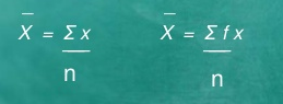
Computation of the mean for ungrouped data
|
Example 1 – The marks obtained in 10 class test are 25, 10, 15, 30, 35

 The mean = X = 25+10+15+30+35 = 115 =23
5 5
Analysis – The average performance of 5 students is 23. The implication is that students who got below 23 did not perform well. The students who got above 23 performed well in exam.
Example 2 – Find the mean
Xi | 9 | 10 | 11 | 12 | 13 | 14 | 15 |
Freq (Fi) | 2 | 5 | 12 | 17 | 14 | 6 | 3 |
Xi | Freq (Fi) | XiFi |
9 | 2 | 18 |
10 | 5 | 50 |
11 | 12 | 132 |
12 | 17 | 204 |
13 | 14 | 182 |
14 | 6 | 84 |
15 | 3 | 45 |
| Fi = 59 | XiFi= 715 |
|
|
|
Then, N = ∑ fi = 59, and ∑fi Xi=715
 X = 715/59 = 12.11
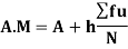
Mean for grouped data/ Weighted Arithmetic Mean
Grouped data are the data that are arranged in a frequency distribution
Frequency distribution is the arrangement of scores according to category of classes including the frequency.
Frequency is the number of observations falling in a category
The formula in solving the mean for grouped data is called midpoint method. The formula is
|
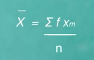
 Where, X = Mean
Xm = midpoint of each class or category
f = frequency in each class or category
∑f Xm = summation of the product of fXm
Example 3 – the following data represent the income distribution of 100 families. Calculate mean income of 100 families?
Income | 30-40 | 40-50 | 50-60 | 60-70 | 70-80 | 80-90 | 90-100 |
No. of families | 8 | 12 | 25 | 22 | 16 | 11 | 6 |
Solution:
Income | No. of families | Xm (Mid point) | fXm |
30-40 | 8 | 35 | 280 |
40-50 | 12 | 34 | 408 |
50-60 | 25 | 55 | 1375 |
60-70 | 22 | 65 | 1430 |
70-80 | 16 | 75 | 1200 |
80-90 | 11 | 85 | 935 |
90-100 | 6 | 95 | 570 |
| n = 100 |
| ∑f Xm = 6198 |

X = ∑f Xm/n = 6330/100 = 63.30
Mean = 63.30
Example 4 – Calculate the mean number of hours per week spent by each student in texting message.
Time per week | 0 – 5 | 5 – 10 | 10 - 15 | 15 - 20 | 20 – 25 | 25 – 30 |
No. of students | 8 | 11 | 15 | 12 | 9 | 5 |
Solution:
Time per week (X) | No. of students (F) | Midpoint X | XF |
0 - 5 | 8 | 2.5 | 20 |
5 – 10 | 11 | 7.5 | 82.5 |
10 - 15 | 15 | 12.5 | 187.5 |
15 - 20 | 12 | 17.5 | 210 |
20 - 25 | 9 | 22.5 | 202.5 |
25 – 30 | 5 | 27.5 | 137.5 |
| 60 |
| 840 |
Mean = 840/60 = 14
Example 5 –
The following table of grouped data represents the weights (in pounds) of all 100 babies born at a local hospital last year.
Weight (pounds) | Number of Babies |
[3−5) | 8 |
[5−7) | 25 |
[7−9) | 45 |
[9−11) | 18 |
[11−13) | 4 |
Solution:
Weight (pounds) | Number of Babies | Midpoint X | XF |
[3−5) | 8 | 4 | 32 |
[5−7) | 25 | 6 | 150 |
[7−9) | 45 | 8 | 360 |
[9−11) | 18 | 10 | 180 |
[11−13) | 4 | 12 | 48 |
| 100 |
| 770 |
Mean = 770/100 = 7.7
Mode
The mode is denoted Mo, is the value which occurs most frequently in a set of values.
Croxton and Cowden defined it as “the mode of a distribution is the value at the point armed with the item tends to most heavily concentrated. It may be regarded as the most typical of a series of value”
Mode for ungrouped data
Example 1- Find the mode of scores of section A
Scores = 25, 24, 24, 20, 17, 18, 10, 18, 9, 7
Solution – Mode is 24, 18 as both have occurred twice.
Mode for grouped data
 Mode = L1 + (L2 – L1) d1
d1 +d2
L1= lower limit of the modal class,
L2= upper limit of the modal class‟
d1 =fm-f0 and d2=fm-f1
Where fm= frequency of the modal class,
f0 = frequency of the class preceding to the modal class,
f1= frequency of the class succeeding to the modal class.
Example 2 – Find the mode
Seconds | Frequency |
51 - 55 | 2 |
56 - 60 | 7 |
61 - 65 | 8 |
66 - 70 | 4 |
Solution
The group with the highest frequency is the modal group: - 61-65
D1 = 8-7 = 1
D2 = 8-4 = 4
 Mode = L1 + (L2 – L1) d1
d1 +d2
 mode = 61 + (65-61) 1 = 61+4 (1/5) = 61.8
1+4
Mode = 61.8
Example 3 - In a class of 30 students marks obtained by students in science out of 50 is tabulated below. Calculate the mode of the given data
Marks obtained | No. of students |
10 -20 | 5 |
20 – 30 | 12 |
30 – 40 | 8 |
40 – 50 | 5 |
Solution:
The group with the highest frequency is the modal group: - 20 -30
D1 = 12 - 5 = 7
D2 = 12 - 8 = 4
 Mode = L1 + (L2 – L1) d1
d1 +d2
 mode = 20 + (30-20) 7 = 20+10 (7/11) = 26.36
7+4
Mode = 61.8
Example 4- Based on the group data below, find the mode
Time to travel to work | Frequency |
1 – 10 | 8 |
11 -20 | 14 |
21 – 30 | 12 |
31 – 40 | 9 |
41 – 50 | 7 |
Solution:
The group with the highest frequency is the modal group: - 11 - 20
D1 = 14 - 8 = 6
D2 = 14 - 12 = 2
 Mode = L1 + (L2 – L1) d1
d1 +d2
 mode = 11 + (20-11) 6 = 11+9 (6/8) = 17.75
6+2
Example 5 –
Compute the mode from the following frequency distribution
CI | F |
70-71 | 2 |
68-69 | 2 |
66-67 | 3 |
64-65 | 4 |
62-63 | 6 |
60-61 | 7 |
58-59 | 5 |
Solution:
The group with the highest frequency is the modal group: - 60 - 61
D1 = 7 - 6 = 1
D2 = 7 - 5 = 2
 Mode = L1 + (L2 – L1) d1
d1 +d2
 mode = 60 + (61-60) 1 = 60+1 (1/3) 60.85
1+2
Merits of mode
- It is easy to understand & easy to calculate
- It is not affected by extreme values or sampling fluctuations.
- Even if extreme values are not known mode can be calculated.
- It can be located just by inspection in many cases.
- It is always present within the data.
Demerits of mode
- It is not rigidly defined.
- It is not based upon all values of the given data.
- It is not capable of further mathematical treatment.
Median
- The points or value that divides the data into two equal parts
- Firstly , the data are arranged in ascending or descending order .
- The median is the middle number depending on the data size.
- When the data size is odd, the median is the middle value
- When the data size is even, median is the average of the middle two values
- It is also known as middle score or 50th percentile
 For ungrouped data median is calculated by (n+1)th value
2
Example 1 – find the median score of 7 students in science class
Score = 19, 17, 16, 15, 12, 11, 10
Median = (7+1)/2 = 4th value
Median = 15
Find the median score of 8 students in science class
Score = 19, 17, 16, 15, 12, 11, 10, 9
Median = (8+1)/2 = 4.5th value
Median = (15+12)/2 = 13.5
Example 2 – find the median of the table given below
Marks obtained | No. of students |
20 | 6 |
25 | 20 |
28 | 24 |
29 | 28 |
33 | 15 |
38 | 4 |
42 | 2 |
43 | 1 |
Solution:
Marks obtained | No. of students | cf |
20 | 6 | 6 |
25 | 20 | 26 (20+6) |
28 | 24 | 50 (26+24) |
29 | 28 | 78 |
33 | 15 | 93 |
38 | 4 | 97 |
42 | 2 | 99 |
43 | 1 | 100 |
Median = (n+1)/2 = 100+1/2 = 50.5
Median = (28+29)/2 = 28.5
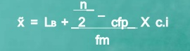
Median of grouped data
Formula
|

 MC = median class is a category containing the n/2
Lb = lower boundary of the median class
Cfp = cumulative frequency before the median class if the scores are arranged from lowest to highest value
Fm = frequency of the median class
c.i = size of the class interval
Ex- calculate the median
Example 3-
Calculate the median
Marks | No. of students |
0-4 | 2 |
5-9 | 8 |
10-14 | 14 |
15-19 | 17 |
20-24 | 9 |
Solution:
Marks | No. of students | CF |
0-4 | 2 | 2 |
5-9 | 8 | 10 |
10-14 | 14 | 24 |
15-19 | 17 | 41 |
20-24 | 9 | 50 |
| 50 |
|
n = 50
 n = 50/2= 25
2
The category containing n/2 is 15 -19
Lb = 15
Cfp = 24
f = 17
ci = 4


|

 Median = 15 + 25-24 *4 = 15.23
17
Example 4 - Given the below frequency table calculate median
X | 60 – 70 | 70 – 80 | 80- 90 | 90-100 |
F | 4 | 5 | 6 | 7 |
Solution:
X | F | CF |
60 - 70 | 4 | 4 |
70 - 80 | 5 | 9 |
80 - 90 | 6 | 15 |
90 - 100 | 7 | 22 |
n = 22
 n = 22/2= 11
2
The category containing n+1/2 is 80 - 90
Lb = 80
Cfp = 9
f = 6
ci = 10
|

 Median = 80 + 11-9 *10 = 83.33
6
Example 5– calculate the median of grouped data
Class interval | 1-3 | 3-5 | 5-7 | 7-9 | 9-11 | 11-13 |
Frequency | 4 | 12 | 13 | 19 | 7 | 5 |
Solution:
CI | F | CF |
1-3 | 4 | 4 |
3-5 | 12 | 16 |
5-7 | 13 | 29 |
7-9 | 19 | 48 |
9-11 | 7 | 55 |
11-13 | 5 | 60 |
n = 60
 n = 60/2= 30
2
The category containing n+1/2 is 7-9
Lb = 7
Cfp = 29
f = 19
ci = 2
|


 Median = 7 + 30-29 *2 = 7.105
19
Merits of median
- It is rigidly defined
- It is easy to understand and easy to calculate
- It is not affected by extreme values
- It is not much affected by sampling fluctuation
- It can be located graphically
Demerits of median
- It is not based upon all values of the given data
- It is difficult to calculate increasing order data size
- It is not capable of further mathematical treatment.
Key takeaways –
- Means is calculated by adding up all the values and divided by the number of observations
- The mode is the value that appears most frequently in a data set.
- the median is the value separating the higher half from the lower half of a data sample

 If there are two groups containing n1 and n2 observations with means x1 and x2 respectively, then the combined arithmetic mean of two groups is given by
|

The above formula can be generalized for more than two groups. If n1 ,n2 ,……,nk are sizes of k groups with means x1, x2 ……., xk respectively then the mean x of the combined group is given by
|

Example 1
If average salaries of two groups of employees are Rs . 1500 and Rs . 2200 and there are 80 and 70 employees in the two groups. Find the mean of the combined group.
Solution
Given : Group I Group II
n1 =80 n2 =70
x1= 1500 x2= 2200
|
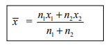
= 80 (1500 ) + 70 (2200)/ 80 +70
= 120000+ 154000/ 150
= 274000/ 150
= 1826.67
The average monthly salary of the combined group of 150 employees is Rs . 1826 .67
Example 2
The mean weight of a group of 50 workers is 58 kgs. The second group consists of 60 workers with average weight 62 kgs. and there are 90 workers in the third group with average weight 56 kgs. Find the average weight of the combined group
Solution
Given Group I Group II Group III
No. of workers n1 =50 n2 =60 n3= 90
Mean weight x1 =58 x2 =62 x3=56
|
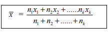
= 50 (58) + 60 (62) + 90 (56)/50 + 60 + 90
= 11660 = 58.3/ 200
∴ The average weight of the combined group of 200 workers is 58.3 kgs
Merits and demerits of measures of central tendency
Merits of Arithmetic Mean.
(1) It is rigidly defined .
(2) It is easy to understand and easy to calculate.
(3) It is based on each and every observation of the series.
(4) It is capable for further mathematical treatment.
(5) It is least affected by sampling fluctuations.
Demerits of Arithmetic Mean.
(1) It is very much affected by extreme observations.
(2) It cannot be used in case of open end classes.
(3) It cannot be determined by inspection nor it can be located graphically.
(4) It cannot be obtained if a single observation is missing .
(5) It is a value which may not be present in the data .
Merits of Median:
- It is rigidly defined.
- It is easy to understand and easy to calculate.
- It is not affected by extreme observations as it is a positional average.
- It can be calculated , even if the extreme values are not known .
- It can be located by mere inspection and can also be located graphically.
- It is the only average to be used while dealing with qualitative characteristics which cannot be measured numerically.
Demerits of Median:
- It is not a good representative in many cases.
- It is not based on all observations.
- It is not capable of further mathematical treatment .
- It is affected by sampling fluctuations.
- For continuous data case , the formula is obtained on the assumption of uniform distribution of frequencies over the class intervals. This assumption may not be true.
Merits of mode
6. It is easy to understand & easy to calculate
7. It is not affected by extreme values or sampling fluctuations.
8. Even if extreme values are not known mode can be calculated.
9. It can be located just by inspection in many cases.
10. It is always present within the data.
Demerits of mode
4. It is not rigidly defined.
5. It is not based upon all values of the given data.
6. It is not capable of further mathematical treatment.
Key takeaways –
- There is a tendency in almost every statistical data that most of the values concentrate at the centre which is referred as ‘central tendency’. The typical values which measure the central tendency are called measures of central tendency.
Geometric mean
Geometric mean is a type of mean or average, which indicates the central tendency of a set of numbers by using the product of their values.
Definition
The Geometric Mean (G.M) of a series containing n observations is the nth root of the product of the values.
For ungrouped data
 Geometric Mean, GM = Antilog ∑logxi
N
Merits of Geometric Mean
- It is rigidly defined.
- It is based on all the items.
- It is capable of further algebraic treatment.
- It gives less weight to large items and more to small items.
Demerits of Geometric Mean
- It is difficult to compute.
- It is not easy to understand.
- If there are negative values in the series, it cannot be computed.
Example 1 – find the G.M of the values
X | Log X |
45 | 1.653 |
60 | 1.778 |
48 | 1.681 |
65 | 1.813 |
Total | 6.925 |
 GM = Antilog ∑logxi
N
= Antilog 6.925/4
= Antilog 1.73
= 53.82
For grouped data
 Geometric Mean, GM = Antilog ∑ f logxi
N
Example 2 – calculate the geometric mean
X | F |
60 – 80 | 22 |
80 – 100 | 38 |
100 – 120 | 45 |
120 – 140 | 35 |
|
|
Solution
X | f | Mid X | Log X | f log X |
60 – 80 | 22 | 70 | 1.845 | 40.59 |
80 – 100 | 38 | 90 | 1.954 | 74.25 |
100 – 120 | 45 | 110 | 2.041 | 91.85 |
120 – 140 | 35 | 130 | 2.114 | 73.99 |
Total | 140 |
|
| 280.68 |
 GM = Antilog ∑ f logxi
N
= antilog 280.68/140
= antilog 2.00
GM = 100
Example 3 – calculate geometric mean
Class | Frequency |
2-4 | 3 |
4-6 | 4 |
6-8 | 2 |
8-10 | 1 |
Solution
Class | frequency | x | Log x | flogx |
2-4 | 3 | 3 | 1.0986 | 3.2958 |
4-6 | 4 | 5 | 1.2875 | 6.4378 |
6-8 | 2 | 7 | 0.5559 | 3.8918 |
8-10 | 1 | 9 | 0.2441 | 2.1972 |
| 10 |
|
| 15.8226 |
 GM = Antilog ∑ f logxi
N
= antilog 15.8226/10
= antilog 1.5823
GM = 4.866
Key takeaways –
- The geometric mean is a mean or average, which indicates the central tendency or typical value of a set of numbers by using the product of their values
Harmonic mean
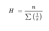
Harmonic mean is quotient of “number of the given values” and “sum of the reciprocals of the given values
For ungrouped data
|
Merits of Harmonic Mean
- It is rigidly defined.
- It is based on all the observations of a series i.e.
- It cannot be calculated ignoring any item of a series.
- It is capable of further algebraic treatment.
Demerits of Harmonic Mean
- It is not easy to understand by a man of ordinary prudence.
- Its calculation is cumbersome as it involves finding out of the reciprocals of the numbers.
- It does not give better and accurate results when the means adopted are the same for the different ends achieved.
- Its algebraic treatment is very much limited and not far and wide as that of the arithmetic mean.
- It is greatly affected by the values of the extreme items.
- It cannot be calculated, if any, of the items is zero.
Example 1 - Calculate the harmonic mean of the numbers 13.2, 14.2, 14.8, 15.2 and 16.1
Solution
X | 1/X |
13.2 | 0.0758 |
14.2 | 0.0704 |
14.8 | 0.0676 |
15.2 | 0.0658 |
16.1 | 0.0621 |
Total | 0.3147 |
H.M of X = 5/0.3147 = 15.88
Example 2 - Find the harmonic mean of the following data {8, 9, 6, 11, 10, 5} ?
X | 1/X |
8 | 0.125 |
9 | 0.111 |
6 | 0.167 |
11 | 0.091 |
10 | 0.100 |
5 | 0.200 |
Total | 0.794 |
H.M of X = 6/0.794 = 7.560
For grouped data
|
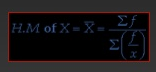
Example 3 - Calculate the harmonic mean for the below data
Marks | 30-39 | 40-49 | 50-59 | 60-69 | 70-79 | 80-89 | 90-99 |
F | 2 | 3 | 11 | 20 | 32 | 25 | 7 |
Solution
Marks | X | F | F/X |
30-39 | 34.5 | 2 | 0.0580 |
40-49 | 44.5 | 3 | 0.0674 |
50-59 | 54.4 | 11 | 0.2018 |
60-69 | 64.5 | 20 | 0.3101 |
70-79 | 74.5 | 32 | 0.4295 |
80-89 | 84.5 | 25 | 0.2959 |
90-99 | 94.5 | 7 | 0.0741 |
Total |
| 100 | 1.4368 |
HM = 100/1.4368 = 69.59
Example 4 – find the harmonic mean of the given class
Ages | 4 | 5 | 6 | 7 |
No. of students | 6 | 4 | 10 | 9 |
Solution
X | F | f/x |
4 | 6 | 1.50 |
5 | 4 | 0.80 |
6 | 10 | 1.67 |
7 | 9 | 1.29 |
| 29.00 | 5.25 |
HM = 29/5.25 = 5.5
Example 5 – calculate harmonic mean
Class | Frequency |
2-4 | 3 |
4-6 | 4 |
6-8 | 2 |
8-10 | 1 |
Solution
Class | frequency | X | f/x |
2-4 | 3 | 3 | 1 |
4-6 | 4 | 5 | 0.8 |
6-8 | 2 | 7 | 0.28 |
8-10 | 1 | 9 | 0.11 |
| 10 |
| 2.19 |
Harmonic mean = 10/2.19 = 4.55
Merits of mean
- It is rigidly defined
- It is easy to understand and easy to calculate
- It is based upon all values of the given data
- It is capable of future mathematical treatment
- It is not much affected by sampling fluctuation
Demerits of mean
- It cannot be calculated if any observation are missing
- It cannot be calculated for open end classes
- It is effected by extreme values
- It cannot be located graphically
- It may be number which is not present in the data
Key takeaways –
- The harmonic mean is a type of numerical average. It is calculated by dividing the number of observations by the reciprocal of each number in the series.
Arithmetic Mean
Arithmetic mean represents a number that is achieved by dividing the sum of the values of a set by the number of values in the set. If a1, a2, a3,….,an, is a number of group of values or the Arithmetic Progression, then;
AM=(a1+a2+a3+….,+an)/n
Geometric Mean
The Geometric Mean for a given number of values containing n observations is the nth root of the product of the values.
GM = n√(a1a2a3….an)
Or
GM = (a1a2a3….an)1/n
Harmonic Mean
HM is defined as the reciprocal of the arithmetic mean of the given data values. It is represented as:
HM = n/[(1/a1) + (1/a2) + (1/a3) + ….+ (1/an)]
The relationship between AM, GM and HM is given by:
AM x HM = GM2
Now let us understand how this relation is derived;
First, consider a, AM, b is an Arithmetic Progression.
Now the common difference of Arithmetic Progression will be;
AM – a = b – AM
a + b = 2 AM …………..(1)
Secondly, let a, GM, b is a Geometric Progression. Then, the common ratio of this GP is;
GM/a = b/GM
ab = GM2……………(2)
Third, is the case of harmonic progression, a, HM, b, where the reciprocals of each term will form an arithmetic progression, such as:
1/a, 1/HM, 1/b is an AP.
Now the common difference of the above AP is;
1/HM – 1/a = 1/b – 1/HM
2/HM = 1/b + 1/a
2/HM = (a + b)/ab ………….(3)
Substituting eq. 1 and eq.2 in eq. 3 we get;
2/HM = 2AM/GM2
GM2 = AM x HM
Hence, this is the relation between Arithmetic, Geometric and Harmonic mean.
Key takeaways –
- The relationship between AM, GM and HM is given by:
AM x HM = GM2
Dispersion is the state of getting dispersed or spread. Statistical dispersion means the extent to which a numerical data is likely to vary about an average value. In other words, dispersion helps to understand the distribution of the data.
Definition
Dispersion is the measures of the variation of the items --- A.L.Bowly
Dispersion is a measure of extent to which the individual items vary --- L.R.Connor
Importance of measuring variation or dispersion
- Testing the Reliability of the Measures of Central Tendency
- Comparing two or more series on the basis of the invariability
- Enabling to control the variability
- Facilitating as a Basis for further statistical Analysis
Characteristics of a Measure of Variation
- It is easy to understand and simple to calculate
- It should be rigidly defined
- It should be based on all observations and it should not be affected by extreme observations
- It should be amenable to further algebraic treatment
- It should have sampling stability
Methods of Measuring Dispersion
- Range
- Inter Quartile range
- Quartile Deviation
- Mean Deviation
- Standard Deviation
- Lorenz Curve
Key takeaways –
- Dispersion is the measures of the variation of the items
- Range – Range defines the difference between the maximum value and the minimum value given in a data set. More the range , group is more variable. The smaller the range the more homogenous is the group.
R = H – L
Example 1 – 5, 10, 15, 20, 7, 9, 17, 13, 12, 16, 8, 6
Range = H-L
=20 – 5 = 15
Coefficient of range –
|
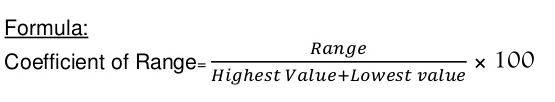
Coefficient of range = (15/(20+5))*100 = 60
Example 2 – what is the range for the following set of numbers?
15,21,57,43,11,39,56,83,77,11,64,91,18,37
Solution
Range = H-L
= 91 – 11 = 80
Therefore the range is 80
Example 3 – the frequency table shows the number of goals the lakers scored in their last twenty matches. What was the range
No. of goals | Frequency |
0 | 2 |
1 | 3 |
2 | 3 |
3 | 6 |
4 | 3 |
5 | 1 |
6 | 1 |
7 | 1 |
Solution
The range is the difference between the lowest and highest values.
The highest value was 7 (They scored 7 goals on 1 occasion)
The lowest value was 0 (They scored 0 goals on 2 occasions)
Therefore the range = 7 - 0 = 7
Example 4 – the following table shows the sales of DVD players made by a retail store each month last year
Month | No. of sales |
January | 25 |
Feb | 43 |
March | 39 |
April | 28 |
May | 29 |
June | 35 |
July | 32 |
August | 46 |
September | 28 |
October | 43 |
November | 51 |
December | 63 |
Solution
The range is the difference between the lowest and highest values.
The lowest number of sales = 25 in January
The highest number of sales = 63 in December
So the range = 63 - 25 = 38
Example 5 – what is the range for the following set of numbers?
57, -5, 11, 39, 56, 82, -2, 11, 64, 18, 37, 15, 68
Solution
The range is the difference between the lowest and highest values.
The highest value is 82.
The lowest value is -5.
Therefore the range = 82 - (-5) = 82+5 = 87
Merits
- Simple and easy to understand
- It gives a quick answer
Demerits
- It is not based on all observation
- Affected by sampling fluctuations
- It cannot be calculated in open ended distributions
2. Interquartile range - the interquartile range measures the range of the middle 50% of the values only. It is calculated as the difference between the upper and lower quartile.
Interquartile range = upper quartile – lower quartile
= Q3 – Q1
Example 1 – find the interquartile range for 1, 2, 18, 6, 7, 9, 27, 15, 5, 19, 12.
Solution
Arrange the numbers in ascending order
1, 2, 5, 6, 7, 9, 12, 15, 18, 19, 27
Find the median
Median = 9
(1, 2, 5, 6, 7), 9, (12, 15, 18, 19, 27)
Q1 as median in the lower half and Q3 as median in the upper half
Q1 = median in (1, 2, 5, 6, 7)
Q1 = 5
Q3 = median in (12, 15, 18, 19, 27)
Q3 = 18
Interquartile range = 18 – 5 = 13
Example 2 – find the interquartile for the following data set: 3, 5, 7, 8, 9, 11, 15, 16, 20, 21.
Solution
Arrange the numbers in ascending order
3, 5, 7, 8, 9, 11, 15, 16, 20, 21
Make a mark in the center of the data:
(3, 5, 7, 8, 9,) | (11, 15, 16, 20, 21)
Find the median
Q1 = 7
Q3 = 16
Interquartile range = 16 – 7 = 9
Example 3 - find the interquartile for the following data set: 1, 3, 4, 5, 5, 6, 7, 11
Make a mark in the center of the data:
(1, 3, 4, 5,) (5, 6, 7, 11)
Find the median
Q1 = (3+4)/2 = 3.5
Q3 = (6+7)/2 = 6.5
Interquartile range = 6.5 – 3.5 = 3
Example 4 -
Find the interquartile range for odd sample size
63,64,64,70,72,76,77,81,81
Solution
Make a mark in the center of the data:
(63,64,64,70,)72,(76,77,81,81)
Find the median
Q1 = (64+64)/2 = 64
Q3 = (77+81)/2 = 79
Interquartile range = 79 – 64 = 15
3. Quartile deviation
Quartile deviation is the product of half of the difference between the upper and the lower quartiles.
QD = (Q3 - Q1) / 2
Coefficient of Quartile Deviation = (Q3 – Q1) / (Q3 + Q1)
Quartile deviation for ungrouped data
|
Examples 1
Day | Frequency |
1 | 20 |
2 | 35 |
3 | 25 |
4 | 12 |
5 | 10 |
6 | 23 |
7 | 18 |
8 | 14 |
9 | 30 |
10 | 40 |
Solution
Arrange the frequency data in ascending order
Day | Frequency |
1 | 10 |
2 | 12 |
3 | 14 |
4 | 18 |
5 | 20 |
6 | 23 |
7 | 25 |
8 | 30 |
9 | 35 |
10 | 40 |
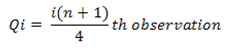
First quartile (Q1)
Qi= [i * (n + 1) /4] th observation
Q1= [1 * (10 + 1) /4] th observation
Q1 = 2.75 th observation
Thus, 2.75 th observation lies between the 2nd and 3rd value in the ordered group, between frequency 12 and 14
First quartile (Q1) is calculated as
Q1 = 2nd observation +0.75 * (3rd observation - 2nd observation)
Q1 = 12 + 0.75 * (14 – 12) = 13.50
Third quartile (Q3)
Qi= [i * (n + 1) /4] th observation
Q3= [3 * (10 + 1) /4] th observation
Q3 = 8.25 th observation
So, 8.25 th observation lies between the 8th and 9th value in the ordered group, between frequency 30 and 35
Third quartile (Q3) is calculated as
Q3 = 8th observation +0.25 * (9th observation – 8th observation)
Q3 = 30 + 0.25 * (35 – 30) = 31.25
Now using the quartiles values Q1 and Q3, we will calculate the quartile deviation.
QD = (Q3 - Q1) / 2
QD = (31.25 – 13.50) / 2 = 8.875
Coefficient of Quartile Deviation = (Q3 – Q1) / (Q3 + Q1)
= (31.25 – 13.50) /(31.25 + 13.50) = 0.397
Example 2 – calculate quartile deviation from the following test scores
Sl. N o | Test scores |
1 | 17 |
2 | 17 |
3 | 26 |
4 | 27 |
5 | 30 |
6 | 30 |
7 | 31 |
8 | 37 |
Solution
First quartile (Q1)
Qi= [i * (n + 1) /4] th observation
Q1= [1 * (8 + 1) /4] th observation
Q1 = 2.25 th observation
Thus, 2.25 th observation lies between the 2nd and 3rd value in the ordered group, between frequency 17 and 26
First quartile (Q1) is calculated as
Q1 = 2nd observation +0.75 * (3rd observation - 2nd observation)
Q1 = 17 + 0.75 * (26 – 17) = 23.75
Third quartile (Q3)
Qi= [i * (n + 1) /4] th observation
Q3= [3 * (8 + 1) /4] th observation
Q3 = 6.75 th observation
So, 6.75 th observation lies between the 6th and 7th value in the ordered group, between frequency 30 and 31
Third quartile (Q3) is calculated as
Q3 = 6th observation +0.25 * (7th observation – 6th observation)
Q3 = 30 + 0.25 * (31 – 30) = 30.25
Now using the quartiles values Q1 and Q3, we will calculate the quartile deviation.
QD = (Q3 - Q1) / 2
QD = (30.25 – 23.75) / 2 = 3.25
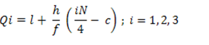
Quartile deviation for grouped data
|

Where,
l = lower boundary of quartile group
h = width of quartile group
f = frequency of quartile group
N = total number of observation
C= cumulative frequency preceding quartile group
Example 3
Age in years | 40 -44 | 45 – 49 | 50 – 54 | 55 - 59 | 60 – 64 | 65 - 69 |
Employees | 5 | 8 | 11 | 10 | 9 | 7 |
Solution
In the case of Frequency Distribution, Quartiles can be calculated by using the formula:
|
Class interval | F | Class boundaries | CF |
40 -44 | 5 | 39.5 – 44.5 | 5 |
45 – 49 | 8 | 44.5 – 49.5 | 13 |
50 – 54 | 11 | 49.5 – 54.5 | 24 |
55 – 59 | 10 | 54.5 – 59.5 | 34 |
60 – 64 | 9 | 59.5 – 64.5 | 43 |
65 – 69 | 7 | 64.5 – 69.5 | 50 |
Total | 50 |
|
|
First quartile (Q1)
Qi= [i * (n ) /4] th observation
Q1 = [1*(50)/4]th observation
Q1 = 12.50th observation
So, 12.50th value is in the interval 44.5 – 49.5
Group of Q1 = 44.5 – 49.5
Qi = (I + (h / f) * ( i * (N/4) – c) ; i = 1,2,3
Q1 = (44.5 + ( 5/ 8)* (1* (50/4) – 5)
Q1 = 49.19
Third quartile (Q3)
Qi= [i * (n) /4] th observation
Q3= [3 * (50) /4] th observation
Q3 = 37.5th observation
So, 37.5th value is in the interval 59.5 – 64.5
Group of Q3 = 59.5 – 64.5
Qi = (I + (h / f) * ( i * (N/4) – c) ; i = 1,2,3
Q3 = (59.5 + ( 5/ 9)* (3* (50/4) – 34)
Q3 = 61.44
QD = (Q3 - Q1) / 2
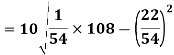
QD = (61.44 – 49.19) / 2 = 6.13
Coefficient of Quartile Deviation = (Q3 – Q1) / (Q3 + Q1)
= (61.44 – 49.19) /(61.44 + 49.19) = 0.11
Example 4 – computation of quartile deviation for grouped test scores
Class | Frequency |
9.3-9.7 | 22 |
9.8-10.2 | 55 |
10.3-10.7 | 12 |
10.8-11.2 | 17 |
11.3-11.7 | 14 |
11.8-12.2 | 66 |
12.3-12.7 | 33 |
12.8-13.2 | 11 |
Solution
Class | Frequency | Class boundaries | CF |
9.3-9.7 | 2 | 9.25-9.75 | 2 |
9.8-10.2 | 5 | 9.75-10.25 | 2 + 5 = 7 |
10.3-10.7 | 12 | 10.25-10.75 | 7 + 12 = 19 |
10.8-11.2 | 17 | 10.75-11.25 | 19 + 17 = 36 |
11.3-11.7 | 14 | 11.25-11.75 | 36 + 14 = 50 |
11.8-12.2 | 6 | 11.75-12.25 | 50 + 6 = 56 |
12.3-12.7 | 3 | 12.25-12.75 | 56 + 3 = 59 |
12.8-13.2 | 1 | 12.75-13.25 | 59 + 1 = 60 |
First quartile (Q1)
Qi= [i * (n ) /4] th observation
Q1 = [1*(60)/4]th observation
Q1 = 15th observation
So, 15th value is in the interval 10.25-10.75
Group of Q1 = 10.25-10.75
Qi = (I + (h / f) * ( i * (N/4) – c) ; i = 1,2,3
Q1 = (10.25 + ( 0.5/ 12)* (1* (60/4) – 7)
Q1 = 10.58
Third quartile (Q3)
Qi= [i * (n) /4] th observation
Q3= [3 * (60) /4] th observation
Q3 = 45th observation
So, 45th value is in the interval 11.25-11.75
Group of Q3 = 11.25-11.75
Qi = (I + (h / f) * ( i * (N/4) – c) ; i = 1,2,3
Q3 = (11.25 + ( 0.5/ 14)* (3* (60/4) – 36)
Q3 = 11.57
QD = (Q3 - Q1) / 2
QD = (11.57 – 10.58) / 2 = 0.495
Example 5 – calculate quartile deviation from the following data
CI | F |
10 – 15 | 6 |
15 – 20 | 10 |
20 – 25 | 15 |
25 – 30 | 22 |
30 – 40 | 12 |
40 – 50 | 9 |
50 – 60 | 4 |
60 – 70 | 2 |
Solution
CI | F | Cf |
10 – 15 | 6 | 6 |
15 – 20 | 10 | 16 |
20 – 25 | 15 | 31 |
25 – 30 | 22 | 53 |
30 – 35 | 12 | 65 |
35 – 40 | 9 | 74 |
45 – 50 | 4 | 78 |
55 – 60 | 2 | 80 |
First quartile (Q1)
Qi= [i * (n ) /4] th observation
Q1 = [1*(80)/4]th observation
Q1 = 20th observation
So, 20th value is in the interval 20 - 25
Group of Q1 = 20 - 25
Qi = (I + (h / f) * ( i * (N/4) – c) ; i = 1,2,3
Q1 = (20 + ( 5/ 15)* (1* (80/4) – 16)
Q1 = 21.33
Third quartile (Q3)
Qi= [i * (n) /4] th observation
Q3= [3 * (80) /4] th observation
Q3 = 60th observation
So, 60th value is in the interval 30 - 35
Group of Q3 = 30 - 35
Qi = (I + (h / f) * ( i * (N/4) – c) ; i = 1,2,3
Q3 = (30 + ( 5/ 12)* (3* (80/4) – 53)
Q3 = 32.91
QD = (Q3 - Q1) / 2
QD = (32.91 – 21.33) / 2 = 5.79
Merits
- It provide better result than range mode
- It is not effected by extreme values
Demerits
- It is completely dependent on central item
- All items are not taken onto consideration
4. Mean deviation – The average of the absolute values of deviation from the mean, median or mode is called mean deviation. This method removes shortcoming of range and QD.
|
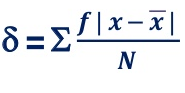
OR
 =
= 
Where, ∑ is total of;
 X is the score, X is the mean, and N is the number of scores
D = Deviation of individual scores from mean
Example 1 –
Computation of mean deviation in ungrouped data
X = 55, 45, 39, 41, 40, 48, 42, 53, 41, 56
Solution
X |
| Absolute deviation (signed ignored) |
55 | 55 - 46 = 9 | 9 |
45 | 45 – 46 = -1 | 1 |
39 | -7 | 7 |
41 | -5 | 5 |
40 | -6 | 6 |
48 | 2 | 2 |
42 | -4 | 4 |
53 | 7 | 7 |
41 | -5 | 5 |
56 | 10 | 10 |
∑X = 460 |
|
|


Mean = 460/10 = 46
MD = 56/10 = 5.6
Example 2- Peter did a survey on the number of pets owned by his classmates, with the following result. What is the mean deviation of the number of pets?
No. of pets | Frequency |
0 | 4 |
1 | 12 |
2 | 8 |
3 | 2 |
4 | 1 |
5 | 2 |
6 | 1 |
Solution
X | F | Fx |
|
|
0 | 4 | 0 | 1.8 | 7.2 |
1 | 12 | 12 | 0.8 | 9.6 |
2 | 8 | 16 | 0.2 | 1.6 |
3 | 2 | 6 | 1.2 | 2.4 |
4 | 1 | 4 | 2.2 | 2.2 |
5 | 2 | 10 | 3.2 | 6.4 |
6 | 1 | 6 | 3.2 | 4.2 |
| 30 | 54 | 4.2 | 33.6 |


Mean = 54/30 = 1.8
MD = 33.6/30 = 1.12
Computation of Mean deviation in grouped data
Example 3 -
Class interval | 15 – 19 | 20 – 24 | 25 – 29 | 30 – 34 | 35 – 39 | 40 – 44 | 45 - 49 |
Frequency | 1 | 4 | 6 | 9 | 5 | 3 | 2 |
Class Interval | F | X | FX | D | FD |
15 – 19 | 1 | 17 | 17 | 15 | 15 |
20 – 24 | 4 | 22 | 88 | 10 | 40 |
25 – 29 | 6 | 27 | 162 | 5 | 30 |
30 – 34 | 9 | 32 | 288 | 0 | 0 |
35 – 39 | 5 | 37 | 185 | 5 | 25 |
40 – 44 | 3 | 42 | 126 | 10 | 30 |
45 – 49 | 2 | 47 | 94 | 15 | 30 |
| N = 30 |
| ∑fx = 960 |
|
|

Mean =960/30 = 32
MD = 170 / 30 = 5.667
Coefficient of mean deviation
|
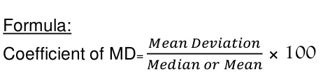
Coefficient of mean deviation = (5.67/32)*100 = 17.71
Example 4 – Calculate mean deviation from the median.
Class | 5 -15 | 15 - 25 | 25 - 35 | 35 - 45 | 45 – 55 |
Frequency | 5 | 9 | 7 | 3 | 8 |
Solution
x | f | cf | Midpoint x | x –median | F(x-m) |
5 -15 | 5 | 5 | 10 | 17.42 | 87.1 |
15 -25 | 9 | 14 | 20 | 7.42 | 66.78 |
25 -35 | 7 | 21 | 30 | 2.58 | 18.06 |
35 -45 | 3 | 24 | 40 | 12.58 | 37.74 |
45- 55 | 8 | 32 | 50 | 22.58 | 180.64 |
| 32 |
|
|
| 390.32 |
Since n/2 = 32/2 = 16, therefore the class is 25 – 35 is the median.
Median =
|

 Median = 25+16-14 *10 = 27.42
7
MD from median is 390.32/32 = 12.91
Example 5 – calculate the mean deviation from continuous frequency distribution
Age group | 15 - 25 | 25 - 35 | 35 - 45 | 45 – 55 |
No. of people | 25 | 54 | 34 | 20 |
Solution
Age group (X) | Number of people (f) | Midpoint x | fx |
|
|
15 – 25 | 25 | 20 | 500 | 13.684 | 324.1 |
25 – 35 | 54 | 30 | 1620 | 3.684 | 198.936 |
35 – 45 | 34 | 40 | 1360 | 6.316 | 214.744 |
45 – 55 | 20 | 50 | 1000 | 16.316 | 352.32 |
| 133 |
|
|
| 1090.1 |


Mean = 4480/133 = 33.684
MD = 1090.1/133 = 8.196
Merits
- It is easy to calculate
- It helps in making comparison
- It is not affected by extreme items
Demerits
- It ignores algebraic sign. And are not used for mathematical treatment
- It is not reliable
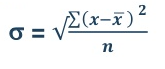
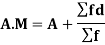
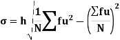
5. Standard deviation – standard deviation is calculated as square root of average of squared deviations taken from actual mean. It is also called root mean square deviation. This measure suffers from less drawbacks and provides accurate results. It removes the drawbacks of ignoring algebraic sign. We square the deviation to make them positive.
Two ways of computing SD
- Direct method
|
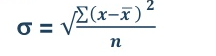
2. Shortcut method
|
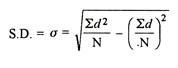
d = Deviation of the score from an assumed mean, say AM; i.e. d = (X – AM). AM is assumed mean
d2 = the square of the deviation.
∑d = the sum of the deviations.
∑d2 = the sum of the squared deviations.
N = No. of the scores
Standard deviation in ungrouped data
- Direct method
Example 1–
X = 12, 15, 10, 8, 11, 13, 18, 10, 14, 9

Mean = 120/10 = 12
Scores | d |
|
12 | 12-12 = 0 | 0 |
15 | 15-12 = 3 | 9 |
10 | 10 -12 = -2 | 4 |
8 | -4 | 16 |
11 | -1 | 1 |
13 | 1 | 1 |
18 | 6 | 36 |
10 | -2 | 4 |
14 | 2 | 4 |
9 | -3 | 9 |
|
|
|


 = 2.9
= 2.9
2. Shortcut method
Assumed mean (AM) = 11
Scores | D = (X- AM) |
|
12 | 12-11 = 1 | 1 |
15 | 15-11 = 4 | 16 |
10 | 10 -11 = -1 | 1 |
8 | -3 | 9 |
11 | 0 | 0 |
13 | 2 | 4 |
18 | 7 | 49 |
10 | --1 | 1 |
14 | 3 | 9 |
9 | -2 | 4 |
|
|
|


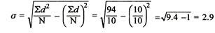
SD from short cut method = 2.9
Example 2 –Ram did a survey of the number of pets owned by his classmates, with the following results
No. of pets | Frequency |
0 | 4 |
1 | 12 |
2 | 8 |
3 | 2 |
4 | 1 |
5 | 2 |
6 | 1 |
Solution
X | f | fx |
|
|
|
0 | 4 | 0 | -1.8 | 3.24 | 12.96 |
1 | 12 | 12 | -0.8 | 0.64 | 7.68 |
2 | 8 | 16 | 0.2 | 0.04 | 0.32 |
3 | 2 | 6 | 1.2 | 1.44 | 2.88 |
4 | 1 | 4 | 2.2 | 4.84 | 4.84 |
5 | 2 | 10 | 3.2 | 10.24 | 20.48 |
6 | 1 | 6 | 4.2 | 17.64 | 17.64 |
| 30 | 54 |
|
| 66.80 |


Mean = 54/30 = 1.8

SD = √66.80/30 = 1.49
Standard deviation in grouped data
Direct method
Example 3 –
C.I. | 0 - 2 | 3 - 5 | 6- 8 | 9-11 | 12-14 | 15 -17 | 18 - 20 |
F | 1 | 3 | 5 | 7 | 6 | 5 | 3 |
Solution
C.I | f | Midpoint x | Fx | D |
| fd2 |
0-2 | 1 | 1 | 1 | -10.1 | 102.01 | 102.01 |
3-5 | 3 | 4 | 12 | -7.1 | 50.41 | 151.23 |
6-8 | 5 | 7 | 35 | -4.1 | 16.81 | 84.05 |
9-11 | 7 | 10 | 70 | -1.1 | 1.21 | 8.47 |
12-14 | 6 | 13 | 78 | 1.9 | 3.61 | 21.66 |
15-17 | 5 | 16 | 80 | 4.9 | 24.01 | 120.05 |
18-20 | 3 | 19 | 57 | 7.9 | 62.41 | 187.23 |
| 30 |
| 333 |
|
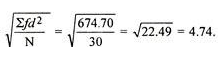
| 674.70 |

Mean = 333/30 = 11.1
SD =
= 
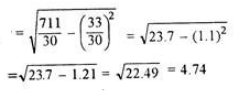
Shortcut method
C.I | F | Midpoint x | d(X-AM) | Fd | fd2 |
0-2 | 1 | 1 | -9 | -9 | 81 |
3-5 | 3 | 4 | -6 | -18 | 108 |
6-8 | 5 | 7 | -3 | -15 | 45 |
9-11 | 7 | 10 | 0 | 0 | 0 |
12-14 | 6 | 13 | 3 | 18 | 54 |
15-17 | 5 | 16 | 6 | 30 | 180 |
18-20 | 3 | 19 | 9 | 27 | 243 |
| 30 |
|
| 33 | 711 |
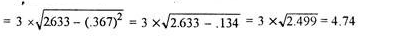
Assumed mean = 10
|

|

Step deviation method
C.I | F | Midpoint x | d | Fd | fd2 |
0-2 | 1 | 1 | -3 | -3 | 9 |
3-5 | 3 | 4 | -2 | -6 | 12 |
6-8 | 5 | 7 | -1 | -5 | 5 |
9-11 | 7 | 10 | 0 | 0 | 0 |
12-14 | 6 | 13 | 1 | 6 | 6 |
15-17 | 5 | 16 | 2 | 10 | 20 |
18-20 | 3 | 19 | 3 | 9 | 27 |
| 30 |
|
| 11 | 79 |
Here, d is calculate as (X –AM)/i, where i is length of class interval
d = (1 -10)/3 = -3 and so on
|
Coefficient of standard deviation
|
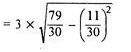
Coefficient of SD = (4.74/11.1)*100 = 42.70
Example 4 – calculate the standard deviation using the direct method
Class interval | Frequency |
30 – 39 | 3 |
40 – 49 | 1 |
50 – 59 | 8 |
60 – 69 | 10 |
70 – 79 | 7 |
80 – 89 | 7 |
90 – 99 | 4 |
Solution
Class interval | Frequency | Midpoint x | fx |
|
|
|
30 – 39 | 3 | 34.5 | 103.5 | -33.5 | 1122.25 | 3366.75 |
40 – 49 | 1 | 44.5 | 44.5 | -23.5 | 552.25 | 552.25 |
50 – 59 | 8 | 54.5 | 436.0 | -13.5 | 182.25 | 1458 |
60 – 69 | 10 | 64.5 | 645.0 | -3.5 | 12.25 | 122.5 |
70 – 79 | 7 | 74.5 | 521.5 | 6.5 | 42.25 | 295.75 |
80 – 89 | 7 | 84.5 | 591.5 | 16.5 | 272.25 | 1905.75 |
90 – 99 | 4 | 94.5 | 378.0 | 26.5 | 702.25 | 2809 |
| 40 |
| 2720 |
|
| 10510 |


Mean = 2720/40 = 68

SD = √10510/40 = 16.20
Example 5 - calculate the mean and standard deviation of hours spent watching television by the 220 students.
Hours | No. of students |
10 – 14 | 2 |
15 – 19 | 12 |
20 – 24 | 23 |
25 – 29 | 60 |
30 – 34 | 77 |
35 – 39 | 38 |
40 – 44 | 8 |
Solution
Hours | No. of students | x | fx |
|
|
|
10 – 14 | 2 | 12 | 24 | -17.82 | 317.49 | 634.98 |
15 – 19 | 12 | 17 | 204 | -12.82 | 164.31 | 1971.67 |
20 – 24 | 23 | 22 | 506 | -7.82 | 61.12 | 1405.85 |
25 – 29 | 60 | 27 | 1620 | -2.82 | 7.94 | 476.53 |
30 – 34 | 77 | 32 | 2464 | 2.18 | 4.76 | 366.55 |
35 – 39 | 38 | 37 | 1406 | 7.18 | 51.58 | 1959.98 |
40 – 44 | 8 | 42 | 336 | 12.18 | 148.40 | 1187.17 |
| 220 |
| 6560 |
|
| 8002.73 |


Mean = 6560/220 = 29.82

SD = √8002.73/220 = 6.03
Key takeaways –
- Range is the difference between the highest and the lowest value of frequency for a given frequency distribution.
- The Quartile Deviation (QD) is the product of half of the difference between the upper and. lower quartiles.
- The Standard Deviation is a measure of how spread out numbers are.
- The mean deviation is defined as a statistical measure which is used to calculate the average deviation from the mean value of the given data set.
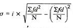
Combined SD
For the combined standard deviation of multiple distributions – X1, X2, X3 … Xk, with individual standard deviations – s1, s2, s3 … sk, arithmetic means – a1, a2, a3 …. ak, and each distribution in turn containing n1, n2, n3 …. nk number of data points, the formula is –
|
Where the summation extends over all the distributions.
In the final formula, di = 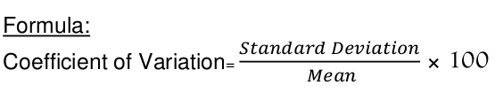
Where, 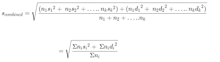 – the arithmetic mean of the i’th distribution
 – the combined arithmetic mean of all distributions, given by –
|

Measures of relative dispersion
Absolute measure of dispersion indicates the amount of variation in a set of values in terms of units of observations. For example, when rainfalls on different days are available in mm, any absolute measure of dispersion gives the variation in rainfall in mm. On the other hand relative measures of dispersion are free from the units of measurements of the observations They are pure numbers. They are used to compare the variation in two or more sets, which are having different units of measurements of observations.
The various absolute and relative measures of dispersion are listed below.
Absolute measure
1. Range
2. Quartile deviation
3. Mean deviation
4. Standard deviation
Relative measure
- Co-efficient of Range
- Co-efficient of Quartile deviation
- Co-efficient of Mean deviation
- Co-efficient of variation
The relative measure corresponding to range, called the coefficient of range, is obtained by applying the following formula:
• Coefficient of Range= (L- S)/ (L S)
Example 1
Find the value of range and its co-efficient for the following data.
7, 9, 6, 8, 11, 10
Solution
L = 11, S = 4.
Range = L – S = 11- 4 = 7
Co-efficient of Range = 𝐿−𝑆 / 𝐿+𝑆
Co-efficient of Range = 11−4/11+4
Co-efficient of Range = 7/15
Co-efficient of Range = 0.4667
Example 2
Calculate range and its co efficient from the following distribution.
Size: 60-63 63-66 66-69 69-72 72-75
Number: 5 18 42 27 8
Solution
L = Upper boundary of the highest class. = 75
S = Lower boundary of the lowest class. = 60
Range = L – S = 75 – 60 = 15
Co-efficient of Range = 𝐿−𝑆/𝐿+S
Co-efficient of Range =75−60/75+60
Co-efficient of Range =15/135
Co-efficient of Range = 0.1111
Example 3
The marks obtained by 9 students are given below:
X = 45 32 37 46 39 36 41 48 36
Calculate coefficient of range
Solution
Co-efficient of Range = 𝐿−𝑆/𝐿+S
Co-efficient of Range =48−32/48+32
Co-efficient of Range =16/80
Co-efficient of Range = 0.2
Key takeaways –
- The coefficient of range on the other hand is the ratio of difference between the highest and lowest value of frequency to the sum of highest and lowest value of frequency.
Coefficient of variation
Formula for calculate Arithmetic Mean (A.M)
Q1) Calculate coefficient variation for the following frequency distribution.
Wages in Rupees earned per day | 0-10 | 10-20 | 20-30 | 30-40 | 40-50 | 50-60 |
No. of Labourers | 5 | 9 | 15 | 12 | 10 | 3 |
A 1)
Wages earned C.I | Mid value | Frequency |
|
|
|
52 | 5 | 5 | -2 | -10 | 20 |
153 | 15 | 9 | -1 | -9 | 9 |
25 | 25 | 15 | 0 | 0 | 0 |
35 | 35 | 12 | 1 | 12 | 12 |
45 | 45 | 10 | 2 | 20 | 40 |
55 | 55 | 3 | 3 | 9 | 27 |
Total | - |
|
|
|
|


Using formula,

 ….. (refer last Ex.)
Now, A.M 
A.M 
 Coefficient of Variation
Q2)
Fluctuations in the aggregate of marks obtained by two groups of students are given below.
Group A | 518 | 519 | 530 | 530 | 530 | 544 | 518 | 550 | 527 | 527 | 531 | 550 | 550 | 529 | 528 |
Group B | 825 | 830 | 830 | 819 | 814 | 814 | 844 | 842 | 826 | 826 | 832 | 835 | 835 | 840 | 840 |
A2) First we represent the data in frequency distribution from group A
|


For group B,
|
|
|
|
|
|
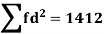
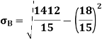
814 819 825 826 830 832 835 840 842 844 | 2 1 1 1 2 1 2 2 2 1 | -16 -11 -5 -4 0 2 5 10 12 14 | 256 121 25 16 0 4 25 100 144 196 | -24 -11 -6 -2 -1 0 1 12 14 60 | 288 121 18 4 1 0 1 144 196 1200 |
Total |
|
|
|
|
|


As we calculate,
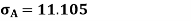
σ for Group A σA=11.105
Now A.M 

A.M 
Coefficient of Variation
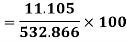

Same for Group B,

Now, 


Coefficient of Variation
Key takeaways –
- The coefficient of variation (CV) is defined as the ratio of the standard deviation to the mean. , It shows the extent of variability in relation to the mean of the population
References
- Practical business mathematics by S.A Bari
- Mathematics of commerce by K. Selvakumar
- Business mathematics with application by Dinesh Khattar and S.R Arora
- Statistical methods by Gupta SP


