Unit 4

Trees

4.1 Tree: Trees and binary trees-concept and terminology

• A Tree is a recursive data structure containing the set of one or more data nodes where one node is designated as the root of the tree while the remaining nodes are called as the children of the root.
• The nodes other than the root node are partitioned into the non empty sets where each one of them is to be called sub-tree.
• Nodes of a tree either maintain a parent-child relationship between them or they are sister nodes.
• In a general tree, A node can have any number of children nodes but it can have only a single parent.
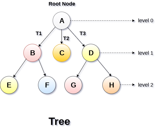
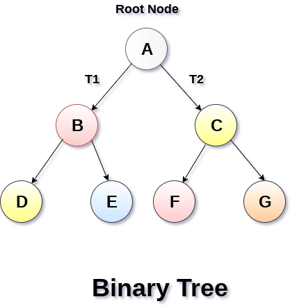
• The following image shows a tree, where the node A is the root node of the tree while the other nodes can be seen as the children of A.

Basic terminology

• Root Node :- The root node is the topmost node in the tree hierarchy. In other words, the root node is the one which doesn't have any parent.
• Sub Tree :- If the root node is not null, the tree T1, T2 and T3 is called sub-trees of the root node.
• Leaf Node :- The node of tree, which doesn't have any child node, is called leaf node. Leaf node is the bottom most node of the tree. There can be any number of leaf nodes present in a general tree. Leaf nodes can also be called external nodes.
• Path :- The sequence of consecutive edges is called path. In the tree shown in the above image, path to the node E is A→ B → E.
• Ancestor node :- An ancestor of a node is any predecessor node on a path from root to that node. The root node doesn't have any ancestors. In the tree shown in the above image, the node F have the ancestors, B and A.
• Degree :- Degree of a node is equal to number of children, a node have. In the tree shown in the above image, the degree of node B is 2. Degree of a leaf node is always 0 while in a complete binary tree, degree of each node is equal to 2.
• Level Number :- Each node of the tree is assigned a level number in such a way that each node is present at one level higher than its parent. Root node of the tree is always present at level 0.

Static representation of tree

1. #define MAXNODE 500  
2. Struct treenode {  
3.    Int root;  
4.    Int father;  
5.    Int son;  
6.    Int next;   
7. }   

Dynamic representation of tree

1. Struct treenode   
2. {  
3.    Int root;  
4.    Struct treenode *father;   
5.    Struct treenode *son   
6.    Struct treenode *next;   
7. }  

Types of Tree

The tree data structure can be classified into six different categories.

General Tree

General Tree stores the elements in a hierarchical order in which the top level element is always present at level 0 as the root element. All the nodes except the root node are present at number of levels. The nodes which are present on the same level are called siblings while the nodes which are present on the different levels exhibit the parent-child relationship among them. A node may contain any number of sub-trees. The tree in which each node contain 3 sub-tree, is called ternary tree.

Forests

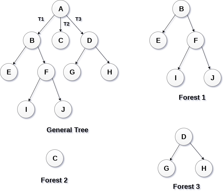
Forest can be defined as the set of disjoint trees which can be obtained by deleting the root node and the edges which connects root node to the first level node.

Binary Tree

Binary tree is a data structure in which each node can have at most 2 children. The node present at the top most level is called the root node. A node with the 0 children is called leaf node. Binary Trees are used in the applications like expression evaluation and many more. We will discuss binary tree in detail, later in this tutorial.

Binary Search Tree

Binary search tree is an ordered binary tree. All the elements in the left sub-tree are less than the root while elements present in the right sub-tree are greater than or equal to the root node element. Binary search trees are used in most of the applications of computer science domain like searching, sorting, etc.

Expression Tree

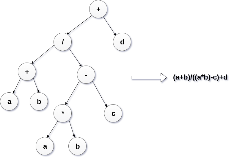
Expression trees are used to evaluate the simple arithmetic expressions. Expression tree is basically a binary tree where internal nodes are represented by operators while the leaf nodes are represented by operands. Expression trees are widely used to solve algebraic expressions like (a+b)*(a-b). Consider the following example.

Q. Construct an expression tree by using the following algebraic expression.

(a + b) / (a*b - c) + d

Tournament Tree

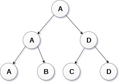
Tournament tree are used to record the winner of the match in each round being played between two players. Tournament tree can also be called as selection tree or winner tree. External nodes represent the players among which a match is being played while the internal nodes represent the winner of the match played. At the top most level, the winner of the tournament is present as the root node of the tree.

For example, tree .of a chess tournament being played among 4 players is shown as follows. However, the winner in the left sub-tree will play against the winner of right sub-tree.

Binary Tree

Binary Tree is a special type of generic tree in which, each node can have at most two children. Binary tree is generally partitioned into three disjoint subsets.

1. Root of the node
2. Left sub-tree which is also a binary tree.
3. Right binary sub-tree

A binary Tree is shown in the following image.

Types of Binary Tree

1. Strictly Binary Tree

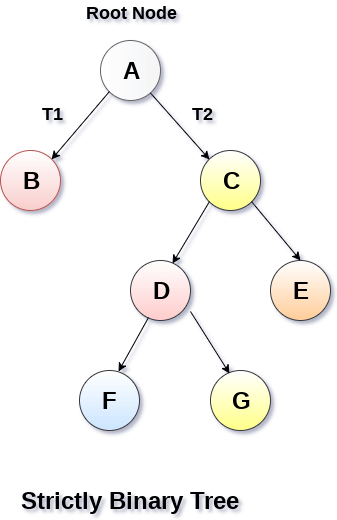
In Strictly Binary Tree, every non-leaf node contain non-empty left and right sub-trees. In other words, the degree of every non-leaf node will always be 2. A strictly binary tree with n leaves, will have (2n - 1) nodes.

A strictly binary tree is shown in the following figure.

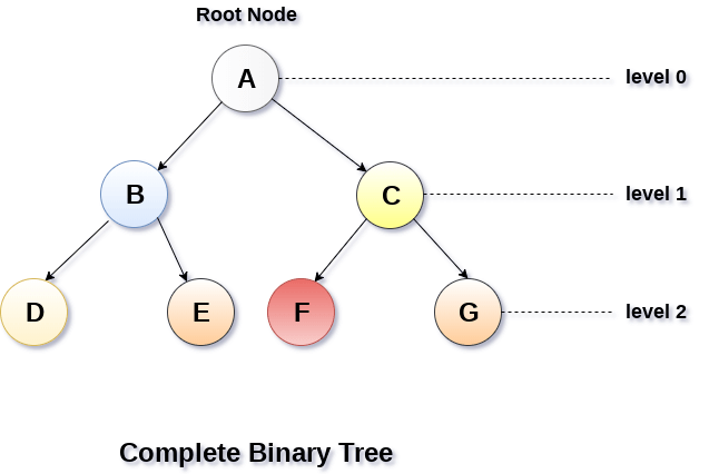
2. Complete Binary Tree

A Binary Tree is said to be a complete binary tree if all of the leaves are located at the same level d. A complete binary tree is a binary tree that contains exactly 2^l nodes at each level between level 0 and d. The total number of nodes in a complete binary tree with depth d is 2d+1-1 where leaf nodes are 2d while non-leaf nodes are 2d-1.

Binary Tree Traversal

Binary Tree representation

There are two types of representation of a binary tree:

1. Linked Representation

In this representation, the binary tree is stored in the memory, in the form of a linked list where the number of nodes are stored at non-contiguous memory locations and linked together by inheriting parent child relationship like a tree. Every node contains three parts : pointer to the left node, data element and pointer to the right node. Each binary tree has a root pointer which points to the root node of the binary tree. In an empty binary tree, the root pointer will point to null.

Consider the binary tree given in the figure below.

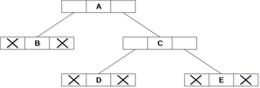
In the above figure, a tree is seen as the collection of nodes where each node contains three parts : left pointer, data element and right pointer. Left pointer stores the address of the left child while the right pointer stores the address of the right child. The leaf node contains null in its left and right pointers.

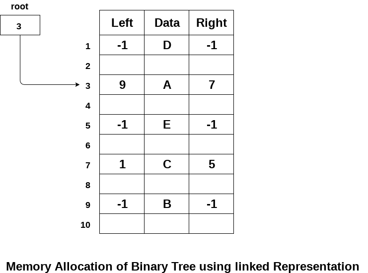
The following image shows about how the memory will be allocated for the binary tree by using linked representation. There is a special pointer maintained in the memory which points to the root node of the tree. Every node in the tree contains the address of its left and right child. Leaf node contains null in its left and right pointers.

2. Sequential Representation

This is the simplest memory allocation technique to store the tree elements but it is an inefficient technique since it requires a lot of space to store the tree elements. A binary tree is shown in the following figure along with its memory allocation.

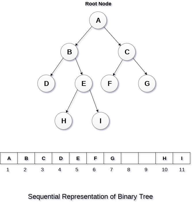
In this representation, an array is used to store the tree elements. Size of the array will be equal to the number of nodes present in the tree. The root node of the tree will be present at the 1st index of the array. If a node is stored at ith index then its left and right children will be stored at 2i and 2i+1 location. If the 1st index of the array i.e. tree[1] is 0, it means that the tree is empty.

4.2 Expression tree

The expression tree is a binary tree in which each internal node corresponds to the operator and each leaf node corresponds to the operand so for example expression tree for 3 + ((5+9)*2) would be:

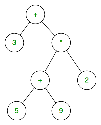
Inorder traversal of expression tree produces infix version of given postfix expression (same with preorder traversal it gives prefix expression)

Evaluating the expression represented by an expression tree: 

Let t be the expression tree

If  t is not null then

If t.value is operand then 

Return  t.value

A = solve(t.left)

B = solve(t.right)

// calculate applies operator 't.value'

// on A and B, and returns value

Return calculate(A, B, t.value)

Construction of Expression Tree: 

Now For constructing an expression tree we use a stack. We loop through input expression and do the following for every character. 

1. If a character is an operand push that into the stack
2. If a character is an operator pop two values from the stack make them its child and push the current node again. 

In the end, the only element of the stack will be the root of an expression tree.

Below is the implementation of the above approach: 

Output

Infix expression is

a + b - e * f * g

4.3 Binary tree as an ADT

A binary tree is defined as a tree in which no node can have more than two children. The highest degree of any node is two. This indicates that the degree of a binary tree is either zero or one or two.

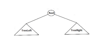
In the above fig., the binary tree consists of a root and two sub trees TreeLeft & TreeRight. All nodes to the left of the binary tree are denoted as left subtrees and all nodes to the right of a binary tree are referred to as right subtrees.

Implementation

A binary tree has maximum two children; we can assign direct pointers to them. The declaration of tree nodes is same as in structure to that for doubly linked lists, in that a node is a structure including the key information plus two pointers (left and right) to other nodes.

Binary Tree node declaration

Typedef struct tree_node *tree_ptr;

Struct tree_node

{

Element_type element1;

Tree_ptr left1; tree_ptr right1;

};

Typedef tree_ptr TREE;

Types of Binary Tree

Strictly binary tree

Strictly binary tree is defined as a binary tree where all the nodes will have either zero or two children. It does not include one child in any node.

Skew tree

A skew tree is defined as a binary tree in which every node except the leaf has only one child node. There are two types of skew tree, i.e. left skewed binary tree and right skewed binary tree.

Left skewed binary tree

A left skew tree has node associated with only the left child. It is a binary tree contains only left subtrees.

Right skewed binary tree

A right skew tree has node associated with only the right child. It is a binary tree contains only right subtrees.

Full binary tree or proper binary tree

A binary tree is defined as a full binary tree if all leaves are at the same level and every non leaf node has exactly two children and it should consist of highest possible number of nodes in all levels. A full binary tree of height h has maximum 2h+1 – 1 nodes.

Complete binary tree

Every non leaf node has exactly two children but all leaves are not necessary to belong at the same level. A complete binary tree is defined as one where all levels have the highest number of nodes except the last level. The last level elements should be filled from left to right direction.

Almost complete binary tree

An almost complete binary tree is defined as a tree in which each node that has a right child also has a left child. Having a left child does not need a node to have a right child

Differences between General Tree and Binary Tree

General Tree

• General tree has no limit of number of children.
• Evaluating any expression is hard in general trees.

Binary Tree

• A binary tree has maximum two children
• Evaluation of expression is simple in binary tree.

Application of trees

• Manipulation of arithmetic expression
• Construction of symbol table
• Analysis of Syntax
• Writing Grammar
• Creation of Expression Tree

4.4 Binary search tree

1. Binary Search tree can be defined as a class of binary trees, in which the nodes are arranged in a specific order. This is also called ordered binary tree.
2. In a binary search tree, the value of all the nodes in the left sub-tree is less than the value of the root.
3. Similarly, value of all the nodes in the right sub-tree is greater than or equal to the value of the root.
4. This rule will be recursively applied to all the left and right sub-trees of the root.

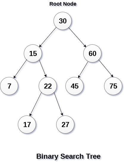
A Binary search tree is shown in the above figure. As the constraint applied on the BST, we can see that the root node 30 doesn't contain any value greater than or equal to 30 in its left sub-tree and it also doesn't contain any value less than 30 in its right sub-tree.

Advantages of using binary search tree

1. Searching become very efficient in a binary search tree since, we get a hint at each step, about which sub-tree contains the desired element.
2. The binary search tree is considered as efficient data structure in compare to arrays and linked lists. In searching process, it removes half sub-tree at every step. Searching for an element in a binary search tree takes o(log2n) time. In worst case, the time it takes to search an element is 0(n).
3. It also speed up the insertion and deletion operations as compare to that in array and linked list.

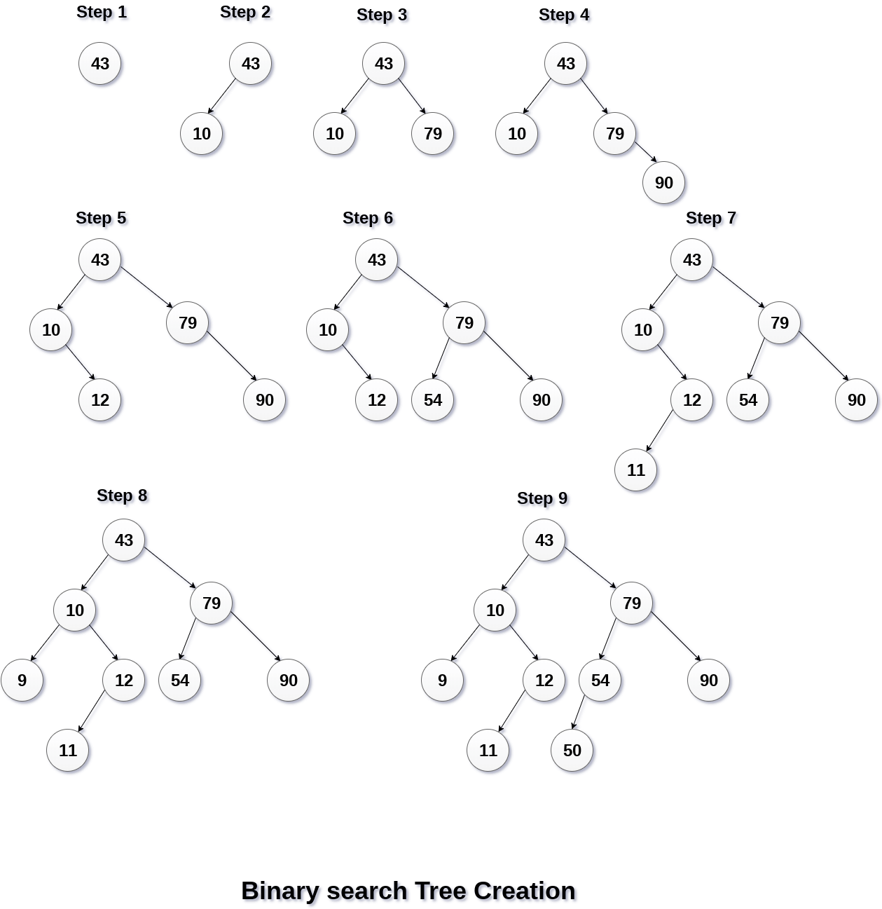
Q. Create the binary search tree using the following data elements.

43, 10, 79, 90, 12, 54, 11, 9, 50

1. Insert 43 into the tree as the root of the tree.
2. Read the next element, if it is lesser than the root node element, insert it as the root of the left sub-tree.
3. Otherwise, insert it as the root of the right of the right sub-tree.

The process of creating BST by using the given elements, is shown in the image below.

Operations on Binary Search Tree

There are many operations which can be performed on a binary search tree.

Program to implement BST operations

1. #include <iostream>  
2. #include <stdlib.h>  
3. Using namespace std;  
4. Struct Node {  
5.    Int data;  
6.    Node *left;  
7.    Node *right;  
8. };  
9. Node* create(int item)  
10. {  
11.    Node* node = new Node;  
12.    Node->data = item;  
13.    Node->left = node->right = NULL;  
14.    Return node;  
15. }  
16.  
17. Void inorder(Node *root)  
18. {  
19.    If (root == NULL)  
20.        Return;  
21.  
22.    Inorder(root->left);  
23.    Cout<< root->data << "   ";  
24.    Inorder(root->right);  
25. }  
26. Node* findMinimum(Node* cur)  
27. {  
28.    While(cur->left != NULL) {  
29.        Cur = cur->left;  
30.    }  
31.    Return cur;  
32. }  
33. Node* insertion(Node* root, int item)  
34. {  
35.    If (root == NULL)  
36.        Return create(item);  
37.    If (item < root->data)  
38.        Root->left = insertion(root->left, item);  
39.    Else  
40.        Root->right = insertion(root->right, item);  
41.  
42.    Return root;  
43. }  
44.  
45. Void search(Node* &cur, int item, Node* &parent)  
46. {  
47.    While (cur != NULL && cur->data != item)  
48.    {  
49.        Parent = cur;  
50.  
51.        If (item < cur->data)  
52.            Cur = cur->left;  
53.        Else  
54.            Cur = cur->right;  
55.    }  
56. }  
57.  
58. Void deletion(Node*& root, int item)  
59. {  
60.    Node* parent = NULL;  
61.    Node* cur = root;  
62.  
63.    Search(cur, item, parent);  
64.    If (cur == NULL)  
65.        Return;  
66.  
67.    If (cur->left == NULL && cur->right == NULL)  
68.    {  
69.        If (cur != root)  
70.        {  
71.            If (parent->left == cur)  
72.                Parent->left = NULL;  
73.            Else  
74.                Parent->right = NULL;  
75.        }  
76.        Else  
77.            Root = NULL;  
78.  
79.        Free(cur);       
80.    }  
81.    Else if (cur->left && cur->right)  
82.    {  
83.        Node* succ  = findMinimum(cur- >right);  
84.  
85.        Int val = succ->data;  
86.  
87.        Deletion(root, succ->data);  
88.  
89.        Cur->data = val;  
90.    }  
91.  
92.    Else  
93.    {  
94.        Node* child = (cur->left)? Cur- >left: cur->right;  
95.  
96.        If (cur != root)  
97.        {  
98.            If (cur == parent->left)  
99.                Parent->left = child;  
100.             Else  
101.                 Parent->right = child;  
102.         }  
103.   
104.         Else  
105.             Root = child;  
106.         Free(cur);  
107.     }  
108. }  
109.   
110. Int main()  
111. {  
112.    Node* root = NULL;  
113.    Int keys[8];  
114.    For(int i=0;i<8;i++)  
115.     {  
116.     Cout << "Enter value to be inserted";  
117.     Cin>>keys[i];  
118.         Root = insertion(root, keys[i]);  
119.     }  
120.   
121.     Inorder(root);  
122.     Cout<<"\n";  
123.     Deletion(root, 10);  
124.     Inorder(root);  
125.     Return 0;  
126. }  

Output:

Enter value to be inserted? 10

Enter value to be inserted? 20

Enter value to be inserted? 30

Enter value to be inserted? 40

Enter value to be inserted?  5

Enter value to be inserted? 25

Enter value to be inserted? 15

Enter value to be inserted?  5

5 5 10 15 20 25 30 40 

5 5 15 20 25 30 40 

4.5 Recursive and Non recursive algorithms for binary tree traversals

Traversal is a common operation performed on data structures. It is the process in which each and every element present in a data structure is "visited" (or accessed) at least once. This may be done to display all of the elements or to perform an operation on all of the elements.

For example, to traverse a singly-linked list, we start with the first (front) node in the list and proceed forward through the list by following the next pointer stored in each node until we reach the end of the list (signified by a next pointer with the special value nullptr). A doubly-linked list can also be traversed in reverse order, starting at the last (back) node in the list and proceeding backwards down the list by following the prev pointer stored in each node, stopping when we reach the beginning of the list (signified by a prev pointer with the special value nullptr). Arrays can likewise easily be traversed either forward or backward, simply by starting with either the first or last element and then incrementing or decrementing a subscript or pointer to the array element.

On the other hand, binary trees can be traversed in multiple ways. These notes describe four different traversals: preorder, inorder, postorder, and level order.

The "Tick Trick"

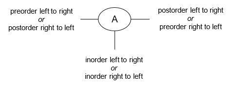
This is a handy trick for figuring out by hand the order in which a binary tree's nodes will be "visited" for the preorder, inorder, and postorder traversals.

1. Draw an arrow as a path around the nodes of the binary tree diagram, closely following its outline. The direction of the arrow depends on whether you are traversing the tree left-to-right or right-to-left.
2. Draw a line or tick mark on one of the sides or the bottom of each node in the tree. Where you draw the mark depends on which traversal you are attempting to perform, as shown in the diagram below:

The point at which the path you've drawn around the binary tree intersects the tick mark is the point at which that node will be "visited" during the traversal.

Preorder Traversal

In a preorder traversal of a binary tree, we "visit" a node and then traverse both of its subtrees. Usually, we traverse the node's left subtree first and then traverse the node's right subtree.

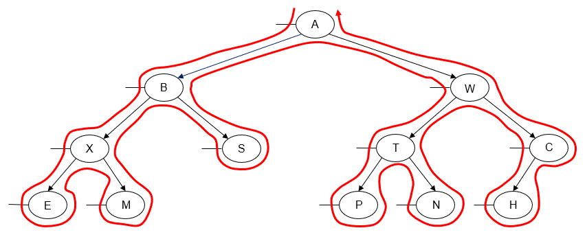
Here's an example of a left-to-right preorder traversal of a binary tree:

Printing the value of each node as we "visit" it, we get the following output:

A B X E M S W T P N C H

Alternatively, we can perform a preorder traversal from right-to-left instead of left-to-right. This is done by traversing the node's right subtree before we traverse its left subtree.

Printing the value of each node as we "visit" it, we get the following output:

A W C H T N P B S X M E

Note that the left-to-right preorder traversal and the right-to-left preorder traversal are not mirror images of each other.

Recursive Preorder Traversal Pseudocode

Given the recursive nature of binary trees (each subtree is itself a binary tree), it's very easy to write preorder traversal as a recursive algorithm. The base case for the recursion occurs when the tree (or subtree) we are attempting to traverse is empty (i.e., the node pointer is nullptr).

Procedure preorder(p : pointer to a tree node)

If p != nullptr

Visit the node pointed to by p

Preorder(p->left)

Preorder(p->right)

End if

End procedure

On the initial call to the preorder() procedure, we pass it the root of the binary tree. To convert the pseudocode above to a right-to-left traversal, just swap left and right so that the right subtree is traversed before the left subtree.

Iterative Preorder Traversal Pseudocode

Preorder traversal can also be performed using a non-recursive or iterative algorithm. In order to backtrack up the tree from a node to its parent, we use a stack.

Procedure iterative_preorder()

// root : pointer to the root node of the tree (nullptr if tree is empty)

// p    : pointer to a tree node

// s    : a stack of pointers to tree nodes

// Start at the root of the tree.

p ← root

// While p is not nullptr or the stack is not empty...

While p != nullptr or s is not empty

// Go all the way to the left.

While p != nullptr

Visit the node pointed to by p

// Place a pointer to the node on the stack before

// traversing the node's left subtree.

s.push(p)

p ← p->left

End while

// p must be nullptr at this point, so backtrack one level.

p ← s.top()

s.pop()

// We have visited the node and its left subtree, so

// now we traverse the node's right subtree.

p ← p->right

End while

End procedure

Inorder Traversal

In an inorder traversal of a binary tree, we traverse one subtree of a node, then "visit" the node, and then traverse its other subtree. Usually, we traverse the node's left subtree first and then traverse the node's right subtree.

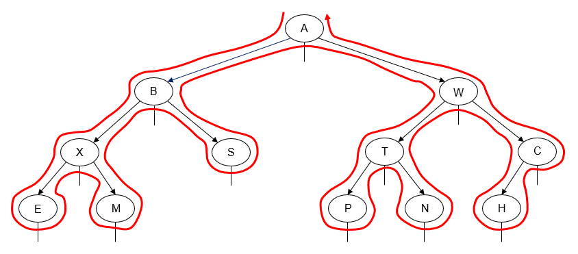
Here's an example of a left-to-right inorder traversal of a binary tree:

Printing the value of each node as we "visit" it, we get the following output:

E X M B S A P T N W H C

Alternatively, we can perform an inorder traversal from right-to-left instead of left-to-right. This is done by traversing the node's right subtree before we traverse its left subtree.

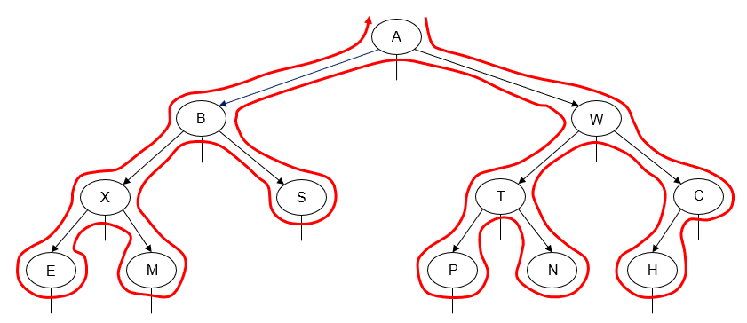
Printing the value of each node as we "visit" it, we get the following output:

C H W N T P A S B M X E

Note that the left-to-right inorder traversal and the right-to-left inorder traversal are mirror images of each other.

Recursive Inorder Traversal Pseudocode

Pseudocode for a recursive inorder traversal is a minor variation of the pseudocode for the recursive preorder traversal:

Procedure inorder(p : pointer to a tree node)

If p != nullptr

Inorder(p->left)

Visit the node pointed to by p

Inorder(p->right)

End if

End procedure

Iterative Inorder Traversal Pseudocode

Inorder traversal can also be performed using a non-recursive or iterative algorithm, in a fashion very similar to the iterative preorder traversal.

Procedure iterative_inorder()

// root : pointer to the root node of the tree (nullptr if tree is empty)

// p    : pointer to a tree node

// s    : a stack of pointers to tree nodes

// Start at the root of the tree.

p ← root

// While p is not nullptr or the stack is not empty...

While p != nullptr or s is not empty

// Go all the way to the left.

While p != nullptr

// Place a pointer to the node on the stack before

// traversing the node's left subtree.

s.push(p)

p ← p->left

End while

// p must be nullptr at this point, so backtrack one level.

p ← s.top()

s.pop()

// We have visited this node's left subtree, so now we

// visit the node.

Visit the node pointed to by p

// We have visited the node and its left subtree, so

// now we traverse the node's right subtree.

p ← p->right

End while

End procedure

Postorder Traversal

In a postorder traversal of a binary tree, we traverse both subtrees of a node, then "visit" the node. Usually we traverse the node's left subtree first and then traverse the node's right subtree.

Here's an example of a left-to-right postorder traversal of a binary tree:

Printing the value of each node as we "visit" it, we get the following output:

E M X S B P N T H C W A

Alternatively, we can perform a postorder traversal from right-to-left instead of left-to-right. Once again, this is done by traversing the node's right subtree before we traverse its left subtree.

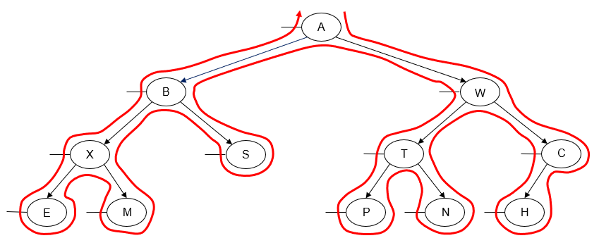
Printing the value of each node as we "visit" it, we get the following output:

H C N P T W S M E X B A

Note that the left-to-right postorder traversal and the right-to-left postorder traversal are not mirror images of each other. However, we can now see that the left-to-right postorder traversal is a mirror image of the right-to-left preorder traversal, while the right-to-left postorder traversal is a mirror image of the left-to-right preorder traversal.

Recursive Postorder Traversal Pseudocode

Once again, pseudocode for a recursive inorder traversal is just a minor variation of the pseudocode for the recursive preorder and inorder traversals:

Procedure postorder(p : pointer to a tree node)

If p != nullptr

Postorder(p >left)

Postorder(p->right)

Visit the node pointed to by p

End if

End procedure

Iterative Postorder Traversal Pseudocode

Postorder traversal can also be performed using a non-recursive or iterative algorithm. This is a trickier algorithm to write than the iterative preorder or inorder traversals, since we will need to backtrack from a node to its parent twice. Some sources solve this problem (poorly, in my opinion) by using two different stacks. Donald Knuth's The Art of Computer Programming has a more efficient version of the algorithm that maintains an extra pointer to the node that was last visited and uses it to distinguish between backtracking to a node after traversing its left subtree versus backtracking to a node after traversing its right subtree.

Procedure iterative_postorder()

// root         : pointer to the root node of the tree (nullptr if tree is empty)

// p            : pointer to a tree node

// last_visited : pointer to the last tree node visited

// s            : a stack of pointers to tree nodes

// Start at the root of the tree.

Last_visited ← nullptr

p ← root

While p != nullptr and last_visited != root

// Go all the way to the left.

While p != nullptr and p != last_visited

// Place a pointer to the node on the stack before

// traversing the node's left subtree.

s.push(p)

p ← p->left

End while

// p must be nullptr at this point, so backtrack one

// level.

p ← s.top()

s.pop()

// If this node has no right child or we've already traversed

// its right subtree...

If p->right == nullptr or p->right == last_visited

Visit the node pointed to by p

// Mark this node as the last visited.

Last_visited ← p

Else

// Otherwise, traverse the node's right subtree.

s.push(p)

p ← p->right

End if

End while

End procedure

Level Order Traversal

In a level order traversal of a binary tree, we traverse all of the tree nodes on level 0, then all of the nodes on level 1, etc. The "tick trick" does not work for this traversal, but there's no real need for it, since the order the nodes will be traversed is easy to determine by hand.

Here's an example of a left-to-right level order traversal of a binary tree:

Printing the value of each node as we "visit" it, we get the following output:

A B W X S T C E M P N H

Alternatively, we can perform a level order traversal from right-to-left instead of left-to-right.

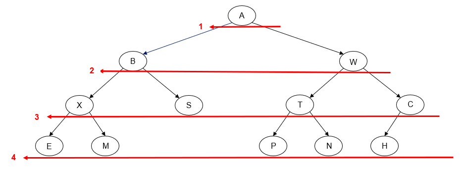
Printing the value of each node as we "visit" it, we get the following output:

A W B C T S X H N P M E

Iterative Level Order Traversal Pseudocode

Level order traversal can be performed using a non-recursive or iterative algorithm. As a given level is traversed, a queue is used to store pointers to the nodes on the next level.

Procedure iterative_level_order()

// root : pointer to the root node of the tree (nullptr if tree is empty)

// p    : pointer to a tree node

// q    : a queue of pointers to tree nodes

// If tree is empty, return.

If root == nullptr

Return

End if

q.push(root)

While q is not empty

// Remove front item in the queue and visit it.

p ← q.front()

q.pop()

Visit the node pointed to by p

// Insert left child of p into queue.

If p->left != nullptr

q.push(p->left)

End if

// Insert right child of p into queue.

If p->right != nullptr

q.push(p->right)

End if

End while

End procedure

Recursive Level Order Traversal Pseudocode

Level order traversal can also be written as a recursive algorithm; here's one example of a solution:

Procedure level_order()

// root : pointer to the root node of the tree (nullptr if tree is empty)

// h    : computed height of the tree (i.e., number of levels

// i    : loop counter

h ← height(root);

i ← 1

While i <= h

Print_level(root, i)

i ← i + 1

End while

End procedure

Procedure print_level(p : pointer to a tree node, level : level number)

If p == nullptr

Return

If level == 1

Visit the node pointed to by p

Else if level > 1

Print_level(p->left, level-1)

Print_level(p->right, level-1)

End if

End procedure

Procedure height(p : pointer to a tree node)

// l_height : computed height of node's left subtree

// r_height : computed height of node's right subtree

If p == nullptr

Return 0

End if

l_height ← height(p->left)

r_height ← height(p->right)

If l_height > r_height

Return l_height + 1

Else

Return r_height + 1

End if

End procedure

The non-recursive algorithm of tree traversals like algorithm for pre-order, post-order and in-order.

1) Algorithm for Post order

In this traversal first, traverse the leftmost subtree at the external node then visit the root node and lastly traverse the right subtree starting at the left external node.

POSTORD(INFO, LEFT, RIGHT, ROOT)

Step-1 [Push NULL onto STACK and initialize PTR]

Set TOP=1, STACK[1]=NULL and PTR=ROOT.

Step-2 [Push left-most path onto STACK] repeat step 3 to 5 while PTR not equal NULL.

Step-3 set TOP=TOP+1 and STACK[TOP]=PTR. [Pushes PTR on STACK].

Step-4 if RIGHT[PTR] not equal NULL then [push on STACK.]

Set TOP=TOP+1 and STACK[TOP]= RIGHT[PTR]

[End of if structure]

Step-5 set PTR = LEFT[PTR].[Update pointer PTR]

[End of step 2 loop].

Step-6 set PTR= STACK[TOP] and TOP=TOP-1.

[Pops node from STACK].

Step-7 Repeat while PTR>0;

Apply PROCESS TO INFO[PTR].

Set PTR= STACK[TOP] and TOP= TOP-1.

[Pops node from STACK]

[End of loop]

Step-8 if PTR<0 then:

Set PTR= -PTR

Go to step 2

[End of if structure]

Step-9 Exit.

2) Algorithm for Inorder

In this traversal first traverse, the root node then traverses the left subtree of the external node and lastly traverse the right subtree of the external node.

INORD( INFO, LEFT, RIGHT, ROOT)

Step-1 [Push NULL onto STACK and initialize PTR;]

Set TOP=1 STACK[1]= NULL and PTR=ROOT.

Step-2 Repeat while PTR not equal NULL[Pushes left most path onto STACK].

a) Set TOP=TOP+1 and STACK[TOP]=PTR [saves node]

b) Set PTR=LEFT[PTR] [updates PTR]

[End of loop]

Step-3  set PTR= STACK[TOP and TOP=TOP-1.[pops node from STACK].

Step-4 Repeat step 5 to 7 while PTR is not equal to Null; [backtracking].

Step-5 Apply PROCESS to INFO[PTR],

Step-6 [RIGHT child?] if RIGHT[PTR] is not equal NULL then.

a) Set PTR=RIGHT[PTR]

b) Go to step 3.[End of if structure.]

Step-7 set PTR= STACK[TOP] and TOP=TOP-1. [pops node]

[End of step 4 loop]

Step-8 Exit.

3) Algorithm for Preorder

In this traversal first, traverse all the left external node starting with the leftmost subtree which is then followed by bubble-up all the external node and then traverse the right subtree starting at the left external node which is the followed by bubble-up all the internal nodes and lastly visit the root node.

PREORDER(  INFO, LEFT,RIGHT, ROOT)

Step-1 [initially push NULL onto stack and initialize PTR.]

Set TOP=1 STACK[1]=NULL and PTR= ROOT.

Step-2 Repeat step 3 to 5 while PTR not equal NULL.

Step-3 Apply PROCESS to INFO[PTR].

Step-4 [RIGHT child?]

If RIGHT[PTR] not equal NULL then [PUSH on STACK]

Set TOP= TOP+1 and STACK[TOP]= RIGHT[PTR]

[End of if structure.]

Step-5 [LEFT child?]

If LEFT[PTR] not equal NULL then

Set PTR= LEFT[PTR].

Else [pop from STACK;]

Set PTR= STACK[TOP] and TOP=TOP+!;

[End of if structure]

[End of step 2 loop]

Step-6 Exit.

4.6 Binary search tree as ADT (Insert Search Delete, level wise Display)

Binary search tree is a binary tree in which every node X in the tree, the values of all the keys in its left sub tree are smaller than the key value in X, and the values of all the keys in its right sub tree are larger than the key vale in X.

Comparison between binary tree and binary search tree

Binary tree

A tree is said to be a binary tree if it has atmost two children. It does not have any order.

Binary search tree

A binary search tree is a binary tree in which the key values in the left node is less than the root and the key values in the right node is greater than the root.

Declaration Routine for binary search tree

Struct TreeNode;

Typedef struct Treenode *SearchTree; SearchTree Insert (int X, SearchTree T); SearchTree Delete (int X, SearchTree T); int Find (int X, SearchTree T);

Int FindMin(SearchTree T); int FindMax(SearchTree T);

SearchTree MakeEmpty(SearchTree T); struct TreeNode

{

Int Element; SearchTree Left; SearchTree Right;

};

MakeEmpty

This operation is mainly for initialization when the programmer prefer to initialize the first element as a one node tree.

Routine to make an empty tree

SearchTree MakeEmpty(SearchTree T)

{

If (T!=NULL) {

MakeEmpty(T->Left);

MakeEmpty(T->Right); free(T);

}

Return NULL;

}

Find

This operation requires returning a pointer to the node in tree T that has key X or NULL if there is no such node.

The find operation as follows.

Ø   Check whether the root is NULL if so then return NULL.

Ø   Otherwise, check the value X with the root node value (ie. T->Element)

If X is equal to T->Element, return T

If X is less than T->Element, traverse the left of T recursively.

If X is greater than T->Element, traverse the right of T recursively.

Routine for Find operation

Position Find( ElementType X, SearchTree T )

{

If( T == NULL ) return NULL;

If(X < T->element )

Return( Find( X, T->left ) );

Else

If( X > T->element )

Return( Find( X, T->right ) );

Else

Return T;

}

Example:

To find an element 4 (X = 4) in the below tree

Ø   In the first fig, the element 4 is checked with root 6. 4 is less than 6. So goto the left subtree.

Ø   In the second fig, element 4 is checked with node 2. 4 is greater than 2. So goto the right subtree.

Ø   In the third fig, the element 4 is checked with node 4. The element is equal. So return 4.

FindMin

This operation returns the position of the smallest element in the tree. To find the minimum element, start at the root and go left as long as there is a left child. The stopping point is the smallest element.

Recursive routine for FindMin

Position FindMin( SearchTree T )

{

If( T = = NULL ) return NULL;

Else

If( T->Left = = NULL ) return T;

Else

Return FindMin ( T->Left ) ; }

Non Recursive routine for FindMin

Position FindMin( SearchTree T )

{

If( T != NULL )

{

While(T->Left!=NULL)

{

T = T->Left;

}}

Return T; }

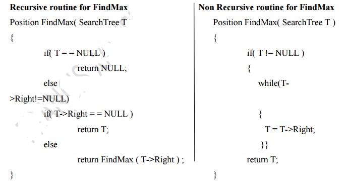
FindMax

This operation returns the position of the largest element in the tree. To find the maximum element, start at the root and go right as long as there is a right child. The stopping point is the largest element.

Insert

Ø   To insert the element X in to the tree, check with the root node T.

Ø   If it is less than the root, traverse the left sub tree recursively until it reaches the T->Left equals to NULL. Then X is placed in T->Left.

Ø   If it is greater than the root, traverse the right sub tree recursively until it reaches the T->Right equals to NULL. Then X is placed in T->Right.

Ø   If X is found in the tree, do nothing.

Recursive routine to insert an element into a binary search tree

SearchTree Insert( ElementType X, SearchTree T )

{

If( T = = NULL )

{ /* Create and return a one-node tree */

T = malloc ( sizeof (struct TreeNode) );

If( T != NULL )

{

T-Element = X;

T->Left = T->Right = NULL;

}}

Else

{

If( X < T->Element )

T->Left = Insert( X, T->Left ); else

If( X > T->Element )

T->Right = Insert( X, T->Right );

/* else X is in the tree already. We'll do nothing */

Return T;

}

Example: To insert 8, 4, 1, 6, 5, 7, 10

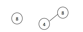
i.        First insert element 8 which is considered as root.

Ii.       Next insert element 4, 4 is less than 8, traverse towards left.

Iii.      Next insert element 1, 1<8 traverse towards left. 1<4 traverse towards left.

Iv.      To insert element 6, 6<8 traverse towards left. 6>4, place it as right child of 4.

v.       To insert element 5, 5<8 traverse towards left. 5>4, traverse towards right. 5<6, place it as left child of 6.

Vi.          To insert element 7, 7<8 traverse towards left. 7>4, traverse towards right. 7>6, place it as right child of 6.

Vii.    To insert element 10, 10>8, place it as a right child of 8.

Delete

While deleting a node from a tree, the memory is to be released. Deletion operation is the complex operation in the binary search tree. To delete a node from the tree consider the following three possibilities.

Case 1: Node to be deleted is a leaf node

Case 2: Node with one child.

Case 3: Node with two children.

Case 1: Deleting the leaf node

Ø   Search the parent of the leaf node.

Ø   Make the parent link of the leaf node as NULL.

Ø   Release Memory.

Example: Deletion of node 6

Case 2: Deleting the node with only one child.

Ø   Search the parent of the node to be deleted.

Ø   Assign the parent link to the child node of the node to be deleted.

Ø   Release the memory of the deleted node.

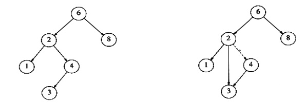
If a node has one child, it can be deleted by adjusting its parent pointer to point to its child node.

Eg: Deletion of a node with one child, before and after

Case 3: Deleting a node with two children.

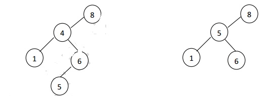
The general strategy is to replace the data of the node to be deleted with its smallest data of the right sub tree (or) largest data of the left sub tree and recursively delete the data or node.

Inorder to delete a node with two children, it can be replaced by a node whose key is larger than any node in P‟s right sub tree to preserve the Binary Search Tree property. The possible nodes that could replace node P are

Rule 1: The node with the largest value in P‟s left sub tree.

Rule 2: The node with the smallest value in P‟s right sub tree.

Eg: Deletion of a node 4 with two children, before and after

Deletion routine for binary search tree

SearchTree Delete( ElementType X, SearchTree T )

{

Position TmpCell;

If( T = = NULL )

Error("Element not found"); else

If( X < T->Element ) /* Go left */

T->Left = Delete( X, T->Left );

Else

If( X > T->Element ) /* Go right */

T->Right = Delete( X, T->Right );

Else    /* Found element to be deleted */

If( T->Left && T->Right ) /* Two children */

{ /* Replace with smallest in right subtree */

TmpCell = FindMin( T->Right );

T->Element = TmpCell->Element;

T->Right = Delete( T->Element, T->Right );

}

Else    /* One or zero child */

{

TmpCell = T;      

If( T->Left = = NULL )  /* Only a right child */

T = T->Right;      

If( T->Right = = NULL )          /* Only a left child */

T = T->Left;        

Free(TmpCell );    

}

Return T;

}

4.7 Threaded binary tree: Concept of threaded binary tree (in order, preorder and post order)

We know that the binary tree nodes may have at most two children. But if they have only one children, or no children, the link part in the linked list representation remains null. Using threaded binary tree representation, we can reuse that empty links by making some threads.

If one node has some vacant left or right child area, that will be used as thread. There are two types of threaded binary tree. The single threaded tree or fully threaded binary tree. In single threaded mode, there are another two variations. Left threaded and right threaded.

In the left threaded mode if some node has no left child, then the left pointer will point to its inorder predecessor, similarly in the right threaded mode if some node has no right child, then the right pointer will point to its inorder successor. In both cases, if no successor or predecessor is present, then it will point to header node.

For fully threaded binary tree, each node has five fields. Three fields like normal binary tree node, another two fields to store Boolean value to denote whether link of that side is actual link or thread.

These are the examples of left and right threaded tree

This is the fully threaded binary tree

4.8 Preorder and In-order traversals of in-order threaded binary tree

Preorder Traversal of Threaded Binary Tree

Algorithm

Make root node as current node.

Until current node is not NULL 

a)Print current key.

b)if current node has left child,then make left child as current node.

c)else if current node has right child then make right child as current node.

d)else

Until right thread exists for current node

Traverse up the right threads and update current.

If current node  = last node.STOP.

Else make right child of current node as current.

Code

Void preorder(node* root)

{

Node* curr = root;

While(curr!=NULL)

{

Printf("%d ",curr->key);

If(curr->left!=NULL)

Curr=curr->left;

Else if(curr->is_rchild==1)

Curr=curr->right;

Else

{

While(curr->right!=NULL && curr->is_rchild==0)      //right thread exists

Curr=curr->right;

If(curr->right == NULL)                            //last node

Break;

Else

Curr=curr->right;

}

}

}

Code Tracing

In order Traversal of a Threaded Binary Tree

Here we will see the threaded binary tree data structure. We know that the binary tree nodes may have at most two children. But if they have only one children, or no children, the link part in the linked list representation remains null. Using threaded binary tree representation, we can reuse that empty links by making some threads.

If one node has some vacant left or right child area, that will be used as thread. There are two types of threaded binary tree. The single threaded tree or fully threaded binary tree.

For fully threaded binary tree, each node has five fields. Three fields like normal binary tree node, another two fields to store Boolean value to denote whether link of that side is actual link or thread.

This is the fully threaded binary tree

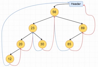
Algorithm

Inorder():

Begin

Temp := root

Repeat infinitely, do

p := temp

Temp = right of temp

If right flag of p is false, then

While left flag of temp is not null, do

Temp := left of temp

Done

End if

If temp and root are same, then

Break

End if

Print key of temp

Done

End

Example

#include <iostream>

#define MAX_VALUE 65536

Using namespace std;

Class N { //node declaration

Public:

Int k;

N *l, *r;

Bool leftTh, rightTh;

};

Class ThreadedBinaryTree {

Private:

N *root;

Public:

ThreadedBinaryTree() { //constructor to initialize the variables

Root= new N();

Root->r= root->l= root;

Root->leftTh = true;

Root->k = MAX_VALUE;

}

Void insert(int key) {

N *p = root;

For (;;) {

If (p->k< key) { //move to right thread

If (p->rightTh)

Break;

p = p->r;

}

Else if (p->k > key) { // move to left thread

If (p->leftTh)

Break;

p = p->l;

}

Else {

Return;

}

}

N *temp = new N();

Temp->k = key;

Temp->rightTh= temp->leftTh= true;

If (p->k < key) {

Temp->r = p->r;

Temp->l= p;

p->r = temp;

p->rightTh= false;

}

Else {

Temp->r = p;

Temp->l = p->l;

p->l = temp;

p->leftTh = false;

}

}

Void inorder() { //print the tree

N *temp = root, *p;

For (;;) {

p = temp;

Temp = temp->r;

If (!p->rightTh) {

While (!temp->leftTh) {

Temp = temp->l;

}

}

If (temp == root)

Break;

Cout<<temp->k<<" ";

}

Cout<<endl;

}

};

Int main() {

ThreadedBinaryTree tbt;

Cout<<"Threaded Binary Tree\n";

Tbt.insert(56);

Tbt.insert(23);

Tbt.insert(89);

Tbt.insert(85);

Tbt.insert(20);

Tbt.insert(30);

Tbt.insert(12);

Tbt.inorder();

Cout<<"\n";

}

Output

Threaded Binary Tree

12 20 23 30 56 85 89

4.9 Applications of trees

Tree Data Structure

In this tutorial, you will learn about tree data structure. Also, you will learn about different types of trees and the terminologies used in tree.

A tree is a nonlinear hierarchical data structure that consists of nodes connected by edges.

A Tree

Why Tree Data Structure?

Other data structures such as arrays, linked list, stack, and queue are linear data structures that store data sequentially. In order to perform any operation in a linear data structure, the time complexity increases with the increase in the data size. But, it is not acceptable in today's computational world.

Different tree data structures allow quicker and easier access to the data as it is a non-linear data structure.

Tree Terminologies

Node

A node is an entity that contains a key or value and pointers to its child nodes.

The last nodes of each path are called leaf nodes or external nodes that do not contain a link/pointer to child nodes.

The node having at least a child node is called an internal node.

Edge

It is the link between any two nodes.

Nodes and edges of a tree

Root

It is the topmost node of a tree.

Height of a Node

The height of a node is the number of edges from the node to the deepest leaf (ie. The longest path from the node to a leaf node).

Depth of a Node

The depth of a node is the number of edges from the root to the node.

Height of a Tree

The height of a Tree is the height of the root node or the depth of the deepest node.

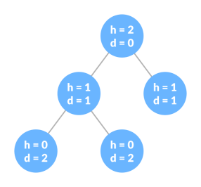
Height and depth of each node in a tree

Degree of a Node

The degree of a node is the total number of branches of that node.

Forest

A collection of disjoint trees is called a forest.

Creating forest from a tree

You can create a forest by cutting the root of a tree.

Types of Tree

1. Binary Tree
2. Binary Search Tree
3. AVL Tree
4. B-Tree

Tree Traversal

In order to perform any operation on a tree, you need to reach to the specific node. The tree traversal algorithm helps in visiting a required node in the tree.

Tree Applications

• Binary Search Trees(BSTs) are used to quickly check whether an element is present in a set or not.
• Heap is a kind of tree that is used for heap sort.
• A modified version of a tree called Tries is used in modern routers to store routing information.
• Most popular databases use B-Trees and T-Trees, which are variants of the tree structure we learned above to store their data
• Compilers use a syntax tree to validate the syntax of every program you write.

References:

1. G. A.V, PAI , “Data Structures and Algorithms “, McGraw Hill, ISBN -13: 978-0-07-066726-6

2. A. Tharp ,"File Organization and Processing", 2008 ,Willey India edition, 9788126518685

3. M. Folk, B. Zoellick, G. Riccardi, "File Structure An Object Oriented Approach with C++", Pearson Education, 2002, ISBN 81 - 7808 - 131 - 8.

4. M. Welss, “Data Structures and Algorithm Analysis in C++", 2nd edition, Pearson Education, 2002, ISBN81-7808-670-0

Unit 4

Trees

4.1 Tree: Trees and binary trees-concept and terminology

• A Tree is a recursive data structure containing the set of one or more data nodes where one node is designated as the root of the tree while the remaining nodes are called as the children of the root.
• The nodes other than the root node are partitioned into the non empty sets where each one of them is to be called sub-tree.
• Nodes of a tree either maintain a parent-child relationship between them or they are sister nodes.
• In a general tree, A node can have any number of children nodes but it can have only a single parent.
• The following image shows a tree, where the node A is the root node of the tree while the other nodes can be seen as the children of A.

Basic terminology

• Root Node :- The root node is the topmost node in the tree hierarchy. In other words, the root node is the one which doesn't have any parent.
• Sub Tree :- If the root node is not null, the tree T1, T2 and T3 is called sub-trees of the root node.
• Leaf Node :- The node of tree, which doesn't have any child node, is called leaf node. Leaf node is the bottom most node of the tree. There can be any number of leaf nodes present in a general tree. Leaf nodes can also be called external nodes.
• Path :- The sequence of consecutive edges is called path. In the tree shown in the above image, path to the node E is A→ B → E.
• Ancestor node :- An ancestor of a node is any predecessor node on a path from root to that node. The root node doesn't have any ancestors. In the tree shown in the above image, the node F have the ancestors, B and A.
• Degree :- Degree of a node is equal to number of children, a node have. In the tree shown in the above image, the degree of node B is 2. Degree of a leaf node is always 0 while in a complete binary tree, degree of each node is equal to 2.
• Level Number :- Each node of the tree is assigned a level number in such a way that each node is present at one level higher than its parent. Root node of the tree is always present at level 0.

Static representation of tree

1. #define MAXNODE 500  
2. Struct treenode {  
3.    Int root;  
4.    Int father;  
5.    Int son;  
6.    Int next;   
7. }   

Dynamic representation of tree

1. Struct treenode   
2. {  
3.    Int root;  
4.    Struct treenode *father;   
5.    Struct treenode *son   
6.    Struct treenode *next;   
7. }  

Types of Tree

The tree data structure can be classified into six different categories.

General Tree

General Tree stores the elements in a hierarchical order in which the top level element is always present at level 0 as the root element. All the nodes except the root node are present at number of levels. The nodes which are present on the same level are called siblings while the nodes which are present on the different levels exhibit the parent-child relationship among them. A node may contain any number of sub-trees. The tree in which each node contain 3 sub-tree, is called ternary tree.

Forests

Forest can be defined as the set of disjoint trees which can be obtained by deleting the root node and the edges which connects root node to the first level node.

Binary Tree

Binary tree is a data structure in which each node can have at most 2 children. The node present at the top most level is called the root node. A node with the 0 children is called leaf node. Binary Trees are used in the applications like expression evaluation and many more. We will discuss binary tree in detail, later in this tutorial.

Binary Search Tree

Binary search tree is an ordered binary tree. All the elements in the left sub-tree are less than the root while elements present in the right sub-tree are greater than or equal to the root node element. Binary search trees are used in most of the applications of computer science domain like searching, sorting, etc.

Expression Tree

Expression trees are used to evaluate the simple arithmetic expressions. Expression tree is basically a binary tree where internal nodes are represented by operators while the leaf nodes are represented by operands. Expression trees are widely used to solve algebraic expressions like (a+b)*(a-b). Consider the following example.

Q. Construct an expression tree by using the following algebraic expression.

(a + b) / (a*b - c) + d

Tournament Tree

Tournament tree are used to record the winner of the match in each round being played between two players. Tournament tree can also be called as selection tree or winner tree. External nodes represent the players among which a match is being played while the internal nodes represent the winner of the match played. At the top most level, the winner of the tournament is present as the root node of the tree.

For example, tree .of a chess tournament being played among 4 players is shown as follows. However, the winner in the left sub-tree will play against the winner of right sub-tree.

Binary Tree

Binary Tree is a special type of generic tree in which, each node can have at most two children. Binary tree is generally partitioned into three disjoint subsets.

1. Root of the node
2. Left sub-tree which is also a binary tree.
3. Right binary sub-tree

A binary Tree is shown in the following image.

Types of Binary Tree

1. Strictly Binary Tree

In Strictly Binary Tree, every non-leaf node contain non-empty left and right sub-trees. In other words, the degree of every non-leaf node will always be 2. A strictly binary tree with n leaves, will have (2n - 1) nodes.

A strictly binary tree is shown in the following figure.

2. Complete Binary Tree

A Binary Tree is said to be a complete binary tree if all of the leaves are located at the same level d. A complete binary tree is a binary tree that contains exactly 2^l nodes at each level between level 0 and d. The total number of nodes in a complete binary tree with depth d is 2d+1-1 where leaf nodes are 2d while non-leaf nodes are 2d-1.

Binary Tree Traversal

Binary Tree representation

There are two types of representation of a binary tree:

1. Linked Representation

In this representation, the binary tree is stored in the memory, in the form of a linked list where the number of nodes are stored at non-contiguous memory locations and linked together by inheriting parent child relationship like a tree. Every node contains three parts : pointer to the left node, data element and pointer to the right node. Each binary tree has a root pointer which points to the root node of the binary tree. In an empty binary tree, the root pointer will point to null.

Consider the binary tree given in the figure below.

In the above figure, a tree is seen as the collection of nodes where each node contains three parts : left pointer, data element and right pointer. Left pointer stores the address of the left child while the right pointer stores the address of the right child. The leaf node contains null in its left and right pointers.

The following image shows about how the memory will be allocated for the binary tree by using linked representation. There is a special pointer maintained in the memory which points to the root node of the tree. Every node in the tree contains the address of its left and right child. Leaf node contains null in its left and right pointers.

2. Sequential Representation

This is the simplest memory allocation technique to store the tree elements but it is an inefficient technique since it requires a lot of space to store the tree elements. A binary tree is shown in the following figure along with its memory allocation.

In this representation, an array is used to store the tree elements. Size of the array will be equal to the number of nodes present in the tree. The root node of the tree will be present at the 1st index of the array. If a node is stored at ith index then its left and right children will be stored at 2i and 2i+1 location. If the 1st index of the array i.e. tree[1] is 0, it means that the tree is empty.

4.2 Expression tree

The expression tree is a binary tree in which each internal node corresponds to the operator and each leaf node corresponds to the operand so for example expression tree for 3 + ((5+9)*2) would be:

Inorder traversal of expression tree produces infix version of given postfix expression (same with preorder traversal it gives prefix expression)

Evaluating the expression represented by an expression tree: 

Let t be the expression tree

If  t is not null then

If t.value is operand then 

Return  t.value

A = solve(t.left)

B = solve(t.right)

// calculate applies operator 't.value'

// on A and B, and returns value

Return calculate(A, B, t.value)

Construction of Expression Tree: 

Now For constructing an expression tree we use a stack. We loop through input expression and do the following for every character. 

1. If a character is an operand push that into the stack
2. If a character is an operator pop two values from the stack make them its child and push the current node again. 

In the end, the only element of the stack will be the root of an expression tree.

Below is the implementation of the above approach: 

Output

Infix expression is

a + b - e * f * g

4.3 Binary tree as an ADT

A binary tree is defined as a tree in which no node can have more than two children. The highest degree of any node is two. This indicates that the degree of a binary tree is either zero or one or two.

In the above fig., the binary tree consists of a root and two sub trees TreeLeft & TreeRight. All nodes to the left of the binary tree are denoted as left subtrees and all nodes to the right of a binary tree are referred to as right subtrees.

Implementation

A binary tree has maximum two children; we can assign direct pointers to them. The declaration of tree nodes is same as in structure to that for doubly linked lists, in that a node is a structure including the key information plus two pointers (left and right) to other nodes.

Binary Tree node declaration

Typedef struct tree_node *tree_ptr;

Struct tree_node

{

Element_type element1;

Tree_ptr left1; tree_ptr right1;

};

Typedef tree_ptr TREE;

Types of Binary Tree

Strictly binary tree

Strictly binary tree is defined as a binary tree where all the nodes will have either zero or two children. It does not include one child in any node.

Skew tree

A skew tree is defined as a binary tree in which every node except the leaf has only one child node. There are two types of skew tree, i.e. left skewed binary tree and right skewed binary tree.

Left skewed binary tree

A left skew tree has node associated with only the left child. It is a binary tree contains only left subtrees.

Right skewed binary tree

A right skew tree has node associated with only the right child. It is a binary tree contains only right subtrees.

Full binary tree or proper binary tree

A binary tree is defined as a full binary tree if all leaves are at the same level and every non leaf node has exactly two children and it should consist of highest possible number of nodes in all levels. A full binary tree of height h has maximum 2h+1 – 1 nodes.

Complete binary tree

Every non leaf node has exactly two children but all leaves are not necessary to belong at the same level. A complete binary tree is defined as one where all levels have the highest number of nodes except the last level. The last level elements should be filled from left to right direction.

Almost complete binary tree

An almost complete binary tree is defined as a tree in which each node that has a right child also has a left child. Having a left child does not need a node to have a right child

Differences between General Tree and Binary Tree

General Tree

• General tree has no limit of number of children.
• Evaluating any expression is hard in general trees.

Binary Tree

• A binary tree has maximum two children
• Evaluation of expression is simple in binary tree.

Application of trees

• Manipulation of arithmetic expression
• Construction of symbol table
• Analysis of Syntax
• Writing Grammar
• Creation of Expression Tree

4.4 Binary search tree

1. Binary Search tree can be defined as a class of binary trees, in which the nodes are arranged in a specific order. This is also called ordered binary tree.
2. In a binary search tree, the value of all the nodes in the left sub-tree is less than the value of the root.
3. Similarly, value of all the nodes in the right sub-tree is greater than or equal to the value of the root.
4. This rule will be recursively applied to all the left and right sub-trees of the root.

A Binary search tree is shown in the above figure. As the constraint applied on the BST, we can see that the root node 30 doesn't contain any value greater than or equal to 30 in its left sub-tree and it also doesn't contain any value less than 30 in its right sub-tree.

Advantages of using binary search tree

1. Searching become very efficient in a binary search tree since, we get a hint at each step, about which sub-tree contains the desired element.
2. The binary search tree is considered as efficient data structure in compare to arrays and linked lists. In searching process, it removes half sub-tree at every step. Searching for an element in a binary search tree takes o(log2n) time. In worst case, the time it takes to search an element is 0(n).
3. It also speed up the insertion and deletion operations as compare to that in array and linked list.

Q. Create the binary search tree using the following data elements.

43, 10, 79, 90, 12, 54, 11, 9, 50

1. Insert 43 into the tree as the root of the tree.
2. Read the next element, if it is lesser than the root node element, insert it as the root of the left sub-tree.
3. Otherwise, insert it as the root of the right of the right sub-tree.

The process of creating BST by using the given elements, is shown in the image below.

Operations on Binary Search Tree

There are many operations which can be performed on a binary search tree.

Program to implement BST operations

1. #include <iostream>  
2. #include <stdlib.h>  
3. Using namespace std;  
4. Struct Node {  
5.    Int data;  
6.    Node *left;  
7.    Node *right;  
8. };  
9. Node* create(int item)  
10. {  
11.    Node* node = new Node;  
12.    Node->data = item;  
13.    Node->left = node->right = NULL;  
14.    Return node;  
15. }  
16.  
17. Void inorder(Node *root)  
18. {  
19.    If (root == NULL)  
20.        Return;  
21.  
22.    Inorder(root->left);  
23.    Cout<< root->data << "   ";  
24.    Inorder(root->right);  
25. }  
26. Node* findMinimum(Node* cur)  
27. {  
28.    While(cur->left != NULL) {  
29.        Cur = cur->left;  
30.    }  
31.    Return cur;  
32. }  
33. Node* insertion(Node* root, int item)  
34. {  
35.    If (root == NULL)  
36.        Return create(item);  
37.    If (item < root->data)  
38.        Root->left = insertion(root->left, item);  
39.    Else  
40.        Root->right = insertion(root->right, item);  
41.  
42.    Return root;  
43. }  
44.  
45. Void search(Node* &cur, int item, Node* &parent)  
46. {  
47.    While (cur != NULL && cur->data != item)  
48.    {  
49.        Parent = cur;  
50.  
51.        If (item < cur->data)  
52.            Cur = cur->left;  
53.        Else  
54.            Cur = cur->right;  
55.    }  
56. }  
57.  
58. Void deletion(Node*& root, int item)  
59. {  
60.    Node* parent = NULL;  
61.    Node* cur = root;  
62.  
63.    Search(cur, item, parent);  
64.    If (cur == NULL)  
65.        Return;  
66.  
67.    If (cur->left == NULL && cur->right == NULL)  
68.    {  
69.        If (cur != root)  
70.        {  
71.            If (parent->left == cur)  
72.                Parent->left = NULL;  
73.            Else  
74.                Parent->right = NULL;  
75.        }  
76.        Else  
77.            Root = NULL;  
78.  
79.        Free(cur);       
80.    }  
81.    Else if (cur->left && cur->right)  
82.    {  
83.        Node* succ  = findMinimum(cur- >right);  
84.  
85.        Int val = succ->data;  
86.  
87.        Deletion(root, succ->data);  
88.  
89.        Cur->data = val;  
90.    }  
91.  
92.    Else  
93.    {  
94.        Node* child = (cur->left)? Cur- >left: cur->right;  
95.  
96.        If (cur != root)  
97.        {  
98.            If (cur == parent->left)  
99.                Parent->left = child;  
100.             Else  
101.                 Parent->right = child;  
102.         }  
103.   
104.         Else  
105.             Root = child;  
106.         Free(cur);  
107.     }  
108. }  
109.   
110. Int main()  
111. {  
112.    Node* root = NULL;  
113.    Int keys[8];  
114.    For(int i=0;i<8;i++)  
115.     {  
116.     Cout << "Enter value to be inserted";  
117.     Cin>>keys[i];  
118.         Root = insertion(root, keys[i]);  
119.     }  
120.   
121.     Inorder(root);  
122.     Cout<<"\n";  
123.     Deletion(root, 10);  
124.     Inorder(root);  
125.     Return 0;  
126. }  

Output:

Enter value to be inserted? 10

Enter value to be inserted? 20

Enter value to be inserted? 30

Enter value to be inserted? 40

Enter value to be inserted?  5

Enter value to be inserted? 25

Enter value to be inserted? 15

Enter value to be inserted?  5

5 5 10 15 20 25 30 40 

5 5 15 20 25 30 40 

4.5 Recursive and Non recursive algorithms for binary tree traversals

Traversal is a common operation performed on data structures. It is the process in which each and every element present in a data structure is "visited" (or accessed) at least once. This may be done to display all of the elements or to perform an operation on all of the elements.

For example, to traverse a singly-linked list, we start with the first (front) node in the list and proceed forward through the list by following the next pointer stored in each node until we reach the end of the list (signified by a next pointer with the special value nullptr). A doubly-linked list can also be traversed in reverse order, starting at the last (back) node in the list and proceeding backwards down the list by following the prev pointer stored in each node, stopping when we reach the beginning of the list (signified by a prev pointer with the special value nullptr). Arrays can likewise easily be traversed either forward or backward, simply by starting with either the first or last element and then incrementing or decrementing a subscript or pointer to the array element.

On the other hand, binary trees can be traversed in multiple ways. These notes describe four different traversals: preorder, inorder, postorder, and level order.

The "Tick Trick"

This is a handy trick for figuring out by hand the order in which a binary tree's nodes will be "visited" for the preorder, inorder, and postorder traversals.

1. Draw an arrow as a path around the nodes of the binary tree diagram, closely following its outline. The direction of the arrow depends on whether you are traversing the tree left-to-right or right-to-left.
2. Draw a line or tick mark on one of the sides or the bottom of each node in the tree. Where you draw the mark depends on which traversal you are attempting to perform, as shown in the diagram below:

The point at which the path you've drawn around the binary tree intersects the tick mark is the point at which that node will be "visited" during the traversal.

Preorder Traversal

In a preorder traversal of a binary tree, we "visit" a node and then traverse both of its subtrees. Usually, we traverse the node's left subtree first and then traverse the node's right subtree.

Here's an example of a left-to-right preorder traversal of a binary tree:

Printing the value of each node as we "visit" it, we get the following output:

A B X E M S W T P N C H

Alternatively, we can perform a preorder traversal from right-to-left instead of left-to-right. This is done by traversing the node's right subtree before we traverse its left subtree.

Printing the value of each node as we "visit" it, we get the following output:

A W C H T N P B S X M E

Note that the left-to-right preorder traversal and the right-to-left preorder traversal are not mirror images of each other.

Recursive Preorder Traversal Pseudocode

Given the recursive nature of binary trees (each subtree is itself a binary tree), it's very easy to write preorder traversal as a recursive algorithm. The base case for the recursion occurs when the tree (or subtree) we are attempting to traverse is empty (i.e., the node pointer is nullptr).

Procedure preorder(p : pointer to a tree node)

If p != nullptr

Visit the node pointed to by p

Preorder(p->left)

Preorder(p->right)

End if

End procedure

On the initial call to the preorder() procedure, we pass it the root of the binary tree. To convert the pseudocode above to a right-to-left traversal, just swap left and right so that the right subtree is traversed before the left subtree.

Iterative Preorder Traversal Pseudocode

Preorder traversal can also be performed using a non-recursive or iterative algorithm. In order to backtrack up the tree from a node to its parent, we use a stack.

Procedure iterative_preorder()

// root : pointer to the root node of the tree (nullptr if tree is empty)

// p    : pointer to a tree node

// s    : a stack of pointers to tree nodes

// Start at the root of the tree.

p ← root

// While p is not nullptr or the stack is not empty...

While p != nullptr or s is not empty

// Go all the way to the left.

While p != nullptr

Visit the node pointed to by p

// Place a pointer to the node on the stack before

// traversing the node's left subtree.

s.push(p)

p ← p->left

End while

// p must be nullptr at this point, so backtrack one level.

p ← s.top()

s.pop()

// We have visited the node and its left subtree, so

// now we traverse the node's right subtree.

p ← p->right

End while

End procedure

Inorder Traversal

In an inorder traversal of a binary tree, we traverse one subtree of a node, then "visit" the node, and then traverse its other subtree. Usually, we traverse the node's left subtree first and then traverse the node's right subtree.

Here's an example of a left-to-right inorder traversal of a binary tree:

Printing the value of each node as we "visit" it, we get the following output:

E X M B S A P T N W H C

Alternatively, we can perform an inorder traversal from right-to-left instead of left-to-right. This is done by traversing the node's right subtree before we traverse its left subtree.

Printing the value of each node as we "visit" it, we get the following output:

C H W N T P A S B M X E

Note that the left-to-right inorder traversal and the right-to-left inorder traversal are mirror images of each other.

Recursive Inorder Traversal Pseudocode

Pseudocode for a recursive inorder traversal is a minor variation of the pseudocode for the recursive preorder traversal:

Procedure inorder(p : pointer to a tree node)

If p != nullptr

Inorder(p->left)

Visit the node pointed to by p

Inorder(p->right)

End if

End procedure

Iterative Inorder Traversal Pseudocode

Inorder traversal can also be performed using a non-recursive or iterative algorithm, in a fashion very similar to the iterative preorder traversal.

Procedure iterative_inorder()

// root : pointer to the root node of the tree (nullptr if tree is empty)

// p    : pointer to a tree node

// s    : a stack of pointers to tree nodes

// Start at the root of the tree.

p ← root

// While p is not nullptr or the stack is not empty...

While p != nullptr or s is not empty

// Go all the way to the left.

While p != nullptr

// Place a pointer to the node on the stack before

// traversing the node's left subtree.

s.push(p)

p ← p->left

End while

// p must be nullptr at this point, so backtrack one level.

p ← s.top()

s.pop()

// We have visited this node's left subtree, so now we

// visit the node.

Visit the node pointed to by p

// We have visited the node and its left subtree, so

// now we traverse the node's right subtree.

p ← p->right

End while

End procedure

Postorder Traversal

In a postorder traversal of a binary tree, we traverse both subtrees of a node, then "visit" the node. Usually we traverse the node's left subtree first and then traverse the node's right subtree.

Here's an example of a left-to-right postorder traversal of a binary tree:

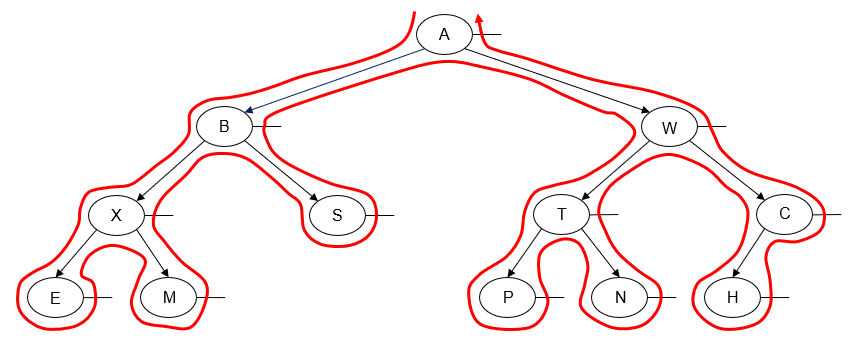
Printing the value of each node as we "visit" it, we get the following output:

E M X S B P N T H C W A

Alternatively, we can perform a postorder traversal from right-to-left instead of left-to-right. Once again, this is done by traversing the node's right subtree before we traverse its left subtree.

Printing the value of each node as we "visit" it, we get the following output:

H C N P T W S M E X B A

Note that the left-to-right postorder traversal and the right-to-left postorder traversal are not mirror images of each other. However, we can now see that the left-to-right postorder traversal is a mirror image of the right-to-left preorder traversal, while the right-to-left postorder traversal is a mirror image of the left-to-right preorder traversal.

Recursive Postorder Traversal Pseudocode

Once again, pseudocode for a recursive inorder traversal is just a minor variation of the pseudocode for the recursive preorder and inorder traversals:

Procedure postorder(p : pointer to a tree node)

If p != nullptr

Postorder(p >left)

Postorder(p->right)

Visit the node pointed to by p

End if

End procedure

Iterative Postorder Traversal Pseudocode

Postorder traversal can also be performed using a non-recursive or iterative algorithm. This is a trickier algorithm to write than the iterative preorder or inorder traversals, since we will need to backtrack from a node to its parent twice. Some sources solve this problem (poorly, in my opinion) by using two different stacks. Donald Knuth's The Art of Computer Programming has a more efficient version of the algorithm that maintains an extra pointer to the node that was last visited and uses it to distinguish between backtracking to a node after traversing its left subtree versus backtracking to a node after traversing its right subtree.

Procedure iterative_postorder()

// root         : pointer to the root node of the tree (nullptr if tree is empty)

// p            : pointer to a tree node

// last_visited : pointer to the last tree node visited

// s            : a stack of pointers to tree nodes

// Start at the root of the tree.

Last_visited ← nullptr

p ← root

While p != nullptr and last_visited != root

// Go all the way to the left.

While p != nullptr and p != last_visited

// Place a pointer to the node on the stack before

// traversing the node's left subtree.

s.push(p)

p ← p->left

End while

// p must be nullptr at this point, so backtrack one

// level.

p ← s.top()

s.pop()

// If this node has no right child or we've already traversed

// its right subtree...

If p->right == nullptr or p->right == last_visited

Visit the node pointed to by p

// Mark this node as the last visited.

Last_visited ← p

Else

// Otherwise, traverse the node's right subtree.

s.push(p)

p ← p->right

End if

End while

End procedure

Level Order Traversal

In a level order traversal of a binary tree, we traverse all of the tree nodes on level 0, then all of the nodes on level 1, etc. The "tick trick" does not work for this traversal, but there's no real need for it, since the order the nodes will be traversed is easy to determine by hand.

Here's an example of a left-to-right level order traversal of a binary tree:

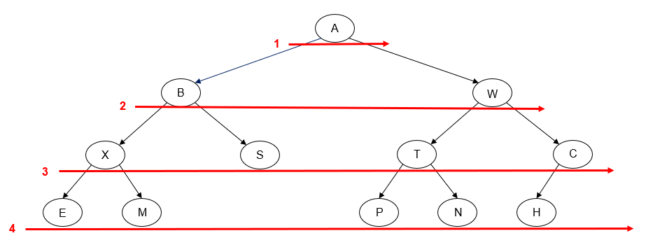
Printing the value of each node as we "visit" it, we get the following output:

A B W X S T C E M P N H

Alternatively, we can perform a level order traversal from right-to-left instead of left-to-right.

Printing the value of each node as we "visit" it, we get the following output:

A W B C T S X H N P M E

Iterative Level Order Traversal Pseudocode

Level order traversal can be performed using a non-recursive or iterative algorithm. As a given level is traversed, a queue is used to store pointers to the nodes on the next level.

Procedure iterative_level_order()

// root : pointer to the root node of the tree (nullptr if tree is empty)

// p    : pointer to a tree node

// q    : a queue of pointers to tree nodes

// If tree is empty, return.

If root == nullptr

Return

End if

q.push(root)

While q is not empty

// Remove front item in the queue and visit it.

p ← q.front()

q.pop()

Visit the node pointed to by p

// Insert left child of p into queue.

If p->left != nullptr

q.push(p->left)

End if

// Insert right child of p into queue.

If p->right != nullptr

q.push(p->right)

End if

End while

End procedure

Recursive Level Order Traversal Pseudocode

Level order traversal can also be written as a recursive algorithm; here's one example of a solution:

Procedure level_order()

// root : pointer to the root node of the tree (nullptr if tree is empty)

// h    : computed height of the tree (i.e., number of levels

// i    : loop counter

h ← height(root);

i ← 1

While i <= h

Print_level(root, i)

i ← i + 1

End while

End procedure

Procedure print_level(p : pointer to a tree node, level : level number)

If p == nullptr

Return

If level == 1

Visit the node pointed to by p

Else if level > 1

Print_level(p->left, level-1)

Print_level(p->right, level-1)

End if

End procedure

Procedure height(p : pointer to a tree node)

// l_height : computed height of node's left subtree

// r_height : computed height of node's right subtree

If p == nullptr

Return 0

End if

l_height ← height(p->left)

r_height ← height(p->right)

If l_height > r_height

Return l_height + 1

Else

Return r_height + 1

End if

End procedure

The non-recursive algorithm of tree traversals like algorithm for pre-order, post-order and in-order.

1) Algorithm for Post order

In this traversal first, traverse the leftmost subtree at the external node then visit the root node and lastly traverse the right subtree starting at the left external node.

POSTORD(INFO, LEFT, RIGHT, ROOT)

Step-1 [Push NULL onto STACK and initialize PTR]

Set TOP=1, STACK[1]=NULL and PTR=ROOT.

Step-2 [Push left-most path onto STACK] repeat step 3 to 5 while PTR not equal NULL.

Step-3 set TOP=TOP+1 and STACK[TOP]=PTR. [Pushes PTR on STACK].

Step-4 if RIGHT[PTR] not equal NULL then [push on STACK.]

Set TOP=TOP+1 and STACK[TOP]= RIGHT[PTR]

[End of if structure]

Step-5 set PTR = LEFT[PTR].[Update pointer PTR]

[End of step 2 loop].

Step-6 set PTR= STACK[TOP] and TOP=TOP-1.

[Pops node from STACK].

Step-7 Repeat while PTR>0;

Apply PROCESS TO INFO[PTR].

Set PTR= STACK[TOP] and TOP= TOP-1.

[Pops node from STACK]

[End of loop]

Step-8 if PTR<0 then:

Set PTR= -PTR

Go to step 2

[End of if structure]

Step-9 Exit.

2) Algorithm for Inorder

In this traversal first traverse, the root node then traverses the left subtree of the external node and lastly traverse the right subtree of the external node.

INORD( INFO, LEFT, RIGHT, ROOT)

Step-1 [Push NULL onto STACK and initialize PTR;]

Set TOP=1 STACK[1]= NULL and PTR=ROOT.

Step-2 Repeat while PTR not equal NULL[Pushes left most path onto STACK].

a) Set TOP=TOP+1 and STACK[TOP]=PTR [saves node]

b) Set PTR=LEFT[PTR] [updates PTR]

[End of loop]

Step-3  set PTR= STACK[TOP and TOP=TOP-1.[pops node from STACK].

Step-4 Repeat step 5 to 7 while PTR is not equal to Null; [backtracking].

Step-5 Apply PROCESS to INFO[PTR],

Step-6 [RIGHT child?] if RIGHT[PTR] is not equal NULL then.

a) Set PTR=RIGHT[PTR]

b) Go to step 3.[End of if structure.]

Step-7 set PTR= STACK[TOP] and TOP=TOP-1. [pops node]

[End of step 4 loop]

Step-8 Exit.

3) Algorithm for Preorder

In this traversal first, traverse all the left external node starting with the leftmost subtree which is then followed by bubble-up all the external node and then traverse the right subtree starting at the left external node which is the followed by bubble-up all the internal nodes and lastly visit the root node.

PREORDER(  INFO, LEFT,RIGHT, ROOT)

Step-1 [initially push NULL onto stack and initialize PTR.]

Set TOP=1 STACK[1]=NULL and PTR= ROOT.

Step-2 Repeat step 3 to 5 while PTR not equal NULL.

Step-3 Apply PROCESS to INFO[PTR].

Step-4 [RIGHT child?]

If RIGHT[PTR] not equal NULL then [PUSH on STACK]

Set TOP= TOP+1 and STACK[TOP]= RIGHT[PTR]

[End of if structure.]

Step-5 [LEFT child?]

If LEFT[PTR] not equal NULL then

Set PTR= LEFT[PTR].

Else [pop from STACK;]

Set PTR= STACK[TOP] and TOP=TOP+!;

[End of if structure]

[End of step 2 loop]

Step-6 Exit.

4.6 Binary search tree as ADT (Insert Search Delete, level wise Display)

Binary search tree is a binary tree in which every node X in the tree, the values of all the keys in its left sub tree are smaller than the key value in X, and the values of all the keys in its right sub tree are larger than the key vale in X.

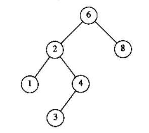
Comparison between binary tree and binary search tree

Binary tree

A tree is said to be a binary tree if it has atmost two children. It does not have any order.

Binary search tree

A binary search tree is a binary tree in which the key values in the left node is less than the root and the key values in the right node is greater than the root.

Declaration Routine for binary search tree

Struct TreeNode;

Typedef struct Treenode *SearchTree; SearchTree Insert (int X, SearchTree T); SearchTree Delete (int X, SearchTree T); int Find (int X, SearchTree T);

Int FindMin(SearchTree T); int FindMax(SearchTree T);

SearchTree MakeEmpty(SearchTree T); struct TreeNode

{

Int Element; SearchTree Left; SearchTree Right;

};

MakeEmpty

This operation is mainly for initialization when the programmer prefer to initialize the first element as a one node tree.

Routine to make an empty tree

SearchTree MakeEmpty(SearchTree T)

{

If (T!=NULL) {

MakeEmpty(T->Left);

MakeEmpty(T->Right); free(T);

}

Return NULL;

}

Find

This operation requires returning a pointer to the node in tree T that has key X or NULL if there is no such node.

The find operation as follows.

Ø   Check whether the root is NULL if so then return NULL.

Ø   Otherwise, check the value X with the root node value (ie. T->Element)

If X is equal to T->Element, return T

If X is less than T->Element, traverse the left of T recursively.

If X is greater than T->Element, traverse the right of T recursively.

Routine for Find operation

Position Find( ElementType X, SearchTree T )

{

If( T == NULL ) return NULL;

If(X < T->element )

Return( Find( X, T->left ) );

Else

If( X > T->element )

Return( Find( X, T->right ) );

Else

Return T;

}

Example:

To find an element 4 (X = 4) in the below tree

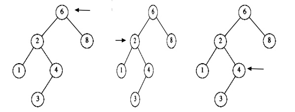
Ø   In the first fig, the element 4 is checked with root 6. 4 is less than 6. So goto the left subtree.

Ø   In the second fig, element 4 is checked with node 2. 4 is greater than 2. So goto the right subtree.

Ø   In the third fig, the element 4 is checked with node 4. The element is equal. So return 4.

FindMin

This operation returns the position of the smallest element in the tree. To find the minimum element, start at the root and go left as long as there is a left child. The stopping point is the smallest element.

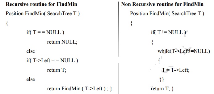
Recursive routine for FindMin

Position FindMin( SearchTree T )

{

If( T = = NULL ) return NULL;

Else

If( T->Left = = NULL ) return T;

Else

Return FindMin ( T->Left ) ; }

Non Recursive routine for FindMin

Position FindMin( SearchTree T )

{

If( T != NULL )

{

While(T->Left!=NULL)

{

T = T->Left;

}}

Return T; }

FindMax

This operation returns the position of the largest element in the tree. To find the maximum element, start at the root and go right as long as there is a right child. The stopping point is the largest element.

Insert

Ø   To insert the element X in to the tree, check with the root node T.

Ø   If it is less than the root, traverse the left sub tree recursively until it reaches the T->Left equals to NULL. Then X is placed in T->Left.

Ø   If it is greater than the root, traverse the right sub tree recursively until it reaches the T->Right equals to NULL. Then X is placed in T->Right.

Ø   If X is found in the tree, do nothing.

Recursive routine to insert an element into a binary search tree

SearchTree Insert( ElementType X, SearchTree T )

{

If( T = = NULL )

{ /* Create and return a one-node tree */

T = malloc ( sizeof (struct TreeNode) );

If( T != NULL )

{

T-Element = X;

T->Left = T->Right = NULL;

}}

Else

{

If( X < T->Element )

T->Left = Insert( X, T->Left ); else

If( X > T->Element )

T->Right = Insert( X, T->Right );

/* else X is in the tree already. We'll do nothing */

Return T;

}

Example: To insert 8, 4, 1, 6, 5, 7, 10

i.        First insert element 8 which is considered as root.

Ii.       Next insert element 4, 4 is less than 8, traverse towards left.

Iii.      Next insert element 1, 1<8 traverse towards left. 1<4 traverse towards left.

Iv.      To insert element 6, 6<8 traverse towards left. 6>4, place it as right child of 4.

v.       To insert element 5, 5<8 traverse towards left. 5>4, traverse towards right. 5<6, place it as left child of 6.

Vi.          To insert element 7, 7<8 traverse towards left. 7>4, traverse towards right. 7>6, place it as right child of 6.

Vii.    To insert element 10, 10>8, place it as a right child of 8.

Delete

While deleting a node from a tree, the memory is to be released. Deletion operation is the complex operation in the binary search tree. To delete a node from the tree consider the following three possibilities.

Case 1: Node to be deleted is a leaf node

Case 2: Node with one child.

Case 3: Node with two children.

Case 1: Deleting the leaf node

Ø   Search the parent of the leaf node.

Ø   Make the parent link of the leaf node as NULL.

Ø   Release Memory.

Example: Deletion of node 6

Case 2: Deleting the node with only one child.

Ø   Search the parent of the node to be deleted.

Ø   Assign the parent link to the child node of the node to be deleted.

Ø   Release the memory of the deleted node.

If a node has one child, it can be deleted by adjusting its parent pointer to point to its child node.

Eg: Deletion of a node with one child, before and after

Case 3: Deleting a node with two children.

The general strategy is to replace the data of the node to be deleted with its smallest data of the right sub tree (or) largest data of the left sub tree and recursively delete the data or node.

Inorder to delete a node with two children, it can be replaced by a node whose key is larger than any node in P‟s right sub tree to preserve the Binary Search Tree property. The possible nodes that could replace node P are

Rule 1: The node with the largest value in P‟s left sub tree.

Rule 2: The node with the smallest value in P‟s right sub tree.

Eg: Deletion of a node 4 with two children, before and after

Deletion routine for binary search tree

SearchTree Delete( ElementType X, SearchTree T )

{

Position TmpCell;

If( T = = NULL )

Error("Element not found"); else

If( X < T->Element ) /* Go left */

T->Left = Delete( X, T->Left );

Else

If( X > T->Element ) /* Go right */

T->Right = Delete( X, T->Right );

Else    /* Found element to be deleted */

If( T->Left && T->Right ) /* Two children */

{ /* Replace with smallest in right subtree */

TmpCell = FindMin( T->Right );

T->Element = TmpCell->Element;

T->Right = Delete( T->Element, T->Right );

}

Else    /* One or zero child */

{

TmpCell = T;      

If( T->Left = = NULL )  /* Only a right child */

T = T->Right;      

If( T->Right = = NULL )          /* Only a left child */

T = T->Left;        

Free(TmpCell );    

}

Return T;

}

4.7 Threaded binary tree: Concept of threaded binary tree (in order, preorder and post order)

We know that the binary tree nodes may have at most two children. But if they have only one children, or no children, the link part in the linked list representation remains null. Using threaded binary tree representation, we can reuse that empty links by making some threads.

If one node has some vacant left or right child area, that will be used as thread. There are two types of threaded binary tree. The single threaded tree or fully threaded binary tree. In single threaded mode, there are another two variations. Left threaded and right threaded.

In the left threaded mode if some node has no left child, then the left pointer will point to its inorder predecessor, similarly in the right threaded mode if some node has no right child, then the right pointer will point to its inorder successor. In both cases, if no successor or predecessor is present, then it will point to header node.

For fully threaded binary tree, each node has five fields. Three fields like normal binary tree node, another two fields to store Boolean value to denote whether link of that side is actual link or thread.

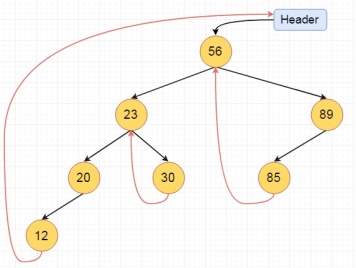
These are the examples of left and right threaded tree

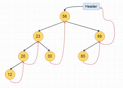
This is the fully threaded binary tree

4.8 Preorder and In-order traversals of in-order threaded binary tree

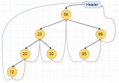
Preorder Traversal of Threaded Binary Tree

Algorithm

Make root node as current node.

Until current node is not NULL 

a)Print current key.

b)if current node has left child,then make left child as current node.

c)else if current node has right child then make right child as current node.

d)else

Until right thread exists for current node

Traverse up the right threads and update current.

If current node  = last node.STOP.

Else make right child of current node as current.

Code

Void preorder(node* root)

{

Node* curr = root;

While(curr!=NULL)

{

Printf("%d ",curr->key);

If(curr->left!=NULL)

Curr=curr->left;

Else if(curr->is_rchild==1)

Curr=curr->right;

Else

{

While(curr->right!=NULL && curr->is_rchild==0)      //right thread exists

Curr=curr->right;

If(curr->right == NULL)                            //last node

Break;

Else

Curr=curr->right;

}

}

}

Code Tracing

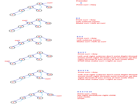
In order Traversal of a Threaded Binary Tree

Here we will see the threaded binary tree data structure. We know that the binary tree nodes may have at most two children. But if they have only one children, or no children, the link part in the linked list representation remains null. Using threaded binary tree representation, we can reuse that empty links by making some threads.

If one node has some vacant left or right child area, that will be used as thread. There are two types of threaded binary tree. The single threaded tree or fully threaded binary tree.

For fully threaded binary tree, each node has five fields. Three fields like normal binary tree node, another two fields to store Boolean value to denote whether link of that side is actual link or thread.

This is the fully threaded binary tree

Algorithm

Inorder():

Begin

Temp := root

Repeat infinitely, do

p := temp

Temp = right of temp

If right flag of p is false, then

While left flag of temp is not null, do

Temp := left of temp

Done

End if

If temp and root are same, then

Break

End if

Print key of temp

Done

End

Example

#include <iostream>

#define MAX_VALUE 65536

Using namespace std;

Class N { //node declaration

Public:

Int k;

N *l, *r;

Bool leftTh, rightTh;

};

Class ThreadedBinaryTree {

Private:

N *root;

Public:

ThreadedBinaryTree() { //constructor to initialize the variables

Root= new N();

Root->r= root->l= root;

Root->leftTh = true;

Root->k = MAX_VALUE;

}

Void insert(int key) {

N *p = root;

For (;;) {

If (p->k< key) { //move to right thread

If (p->rightTh)

Break;

p = p->r;

}

Else if (p->k > key) { // move to left thread

If (p->leftTh)

Break;

p = p->l;

}

Else {

Return;

}

}

N *temp = new N();

Temp->k = key;

Temp->rightTh= temp->leftTh= true;

If (p->k < key) {

Temp->r = p->r;

Temp->l= p;

p->r = temp;

p->rightTh= false;

}

Else {

Temp->r = p;

Temp->l = p->l;

p->l = temp;

p->leftTh = false;

}

}

Void inorder() { //print the tree

N *temp = root, *p;

For (;;) {

p = temp;

Temp = temp->r;

If (!p->rightTh) {

While (!temp->leftTh) {

Temp = temp->l;

}

}

If (temp == root)

Break;

Cout<<temp->k<<" ";

}

Cout<<endl;

}

};

Int main() {

ThreadedBinaryTree tbt;

Cout<<"Threaded Binary Tree\n";

Tbt.insert(56);

Tbt.insert(23);

Tbt.insert(89);

Tbt.insert(85);

Tbt.insert(20);

Tbt.insert(30);

Tbt.insert(12);

Tbt.inorder();

Cout<<"\n";

}

Output

Threaded Binary Tree

12 20 23 30 56 85 89

4.9 Applications of trees

Tree Data Structure

In this tutorial, you will learn about tree data structure. Also, you will learn about different types of trees and the terminologies used in tree.

A tree is a nonlinear hierarchical data structure that consists of nodes connected by edges.

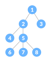
A Tree

Why Tree Data Structure?

Other data structures such as arrays, linked list, stack, and queue are linear data structures that store data sequentially. In order to perform any operation in a linear data structure, the time complexity increases with the increase in the data size. But, it is not acceptable in today's computational world.

Different tree data structures allow quicker and easier access to the data as it is a non-linear data structure.

Tree Terminologies

Node

A node is an entity that contains a key or value and pointers to its child nodes.

The last nodes of each path are called leaf nodes or external nodes that do not contain a link/pointer to child nodes.

The node having at least a child node is called an internal node.

Edge

It is the link between any two nodes.

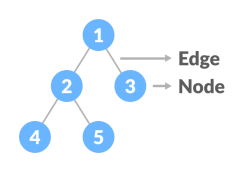
Nodes and edges of a tree

Root

It is the topmost node of a tree.

Height of a Node

The height of a node is the number of edges from the node to the deepest leaf (ie. The longest path from the node to a leaf node).

Depth of a Node

The depth of a node is the number of edges from the root to the node.

Height of a Tree

The height of a Tree is the height of the root node or the depth of the deepest node.

Height and depth of each node in a tree

Degree of a Node

The degree of a node is the total number of branches of that node.

Forest

A collection of disjoint trees is called a forest.

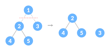
Creating forest from a tree

You can create a forest by cutting the root of a tree.

Types of Tree

1. Binary Tree
2. Binary Search Tree
3. AVL Tree
4. B-Tree

Tree Traversal

In order to perform any operation on a tree, you need to reach to the specific node. The tree traversal algorithm helps in visiting a required node in the tree.

Tree Applications

• Binary Search Trees(BSTs) are used to quickly check whether an element is present in a set or not.
• Heap is a kind of tree that is used for heap sort.
• A modified version of a tree called Tries is used in modern routers to store routing information.
• Most popular databases use B-Trees and T-Trees, which are variants of the tree structure we learned above to store their data
• Compilers use a syntax tree to validate the syntax of every program you write.

References:

1. G. A.V, PAI , “Data Structures and Algorithms “, McGraw Hill, ISBN -13: 978-0-07-066726-6

2. A. Tharp ,"File Organization and Processing", 2008 ,Willey India edition, 9788126518685

3. M. Folk, B. Zoellick, G. Riccardi, "File Structure An Object Oriented Approach with C++", Pearson Education, 2002, ISBN 81 - 7808 - 131 - 8.

4. M. Welss, “Data Structures and Algorithm Analysis in C++", 2nd edition, Pearson Education, 2002, ISBN81-7808-670-0