UNIT 5
BRANCH & BOUND
- The branch and bound algorithm is similar to backtracking but it is used for solving optimization problems i.e. minimization.
- It performs a graph traversed on the state space tree using BFS instead of DFS which is used by backtracking.
- Branch and bound can handle the problem based on discrete and continuous variables.
- Branch and bound is general technique for improving the searching process by systematically enumerating all possible solutions and disposing of obviously impossible solution.
- It has two steps i.e. Branching and bounding
- In branching, there are several choices to be made so that choices branch out into solution space.
- In bounding, it refers to setting a bound on the solution quality also used to reduce the search space.
- Following nodes are used in branch and bound:
- Answer node: Those solution states S for which path from roots to S defines a tuple which is a member of the set of solution of the problem
- Live node: A node which has been generated and all of those children have not yet been generated is live node
- E-node: The live node whose children are currently being generated is called the E node
- Dead node: It is the generated node that is either not to be expanded further or one for which all of its children have been generated.
Branch and bound has following three strategies:
1. BFS is the state space search tree works with FIFO search ie. Live nodes comes first in first out list.
2. DFS is the state space search tree works with LIFO search ie. Live nodes comes last in first out list.
3. Least-cost search
5.2.1 FIFO Search
- BFS with queue based branch and bound is called as FIFO branch & bound
- In FIFO search the children of root node are generated in the first iteration.
- In the next step, children of the first child is generated.
- If the children not already killed by bounding function then put it in the queue, then the children of second child is explored.
Example:
Assume a data structure as Queue. Initially queue is empty.
|
|
|
|
|
|

Assume the node 12 is an answer node (solution)
First take E node as node 1 and take all childerens of node 1 as live nodes.
2 | 3 | 4 |
|
|
|
Now take node 2 and place next childerens in queue.
| 3 | 4 | 5 | 6 |
|
Next delete node 3 and its childeren 7,8 are killed by bounding function.
|
| 4 | 5 | 6 |
|
Delete node 4 and its generated cgildren are killed.
|
|
| 5 | 6 |
|
Next delete element 5 from queue and its children node 10, 11 are generated.
Last node is 6 and its child is 12 which satisfies the solution.
5.2.2 LIFO Branch and Bound Search
Assume data structure as stack. Initially stack is empty.
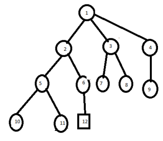
Generate children of node 1 and place them in stack.
|
2 |
3 |
4 |
Remove element from stack ie. Node 2 and place its children
5 |
6 |
3 |
4 |
Again remove one element ie.node 5 and its children are killed by bounded function.
Remove node 6 from stack which generates the solution. Hence search process terminates.
|
6 |
3 |
4 |
5.2.3 Least Cost Search
In the LIFO and FIFO branch and bound the selection rule for the next E node is in sense blind which does not give an preference to node that has very good chance of getting the search to an answer node quickly.
The search for an answer node can often speeded by using an “intelligent ranking function” c ( ) for lives nodes. The next E node is selected on the basis of this ranking function.
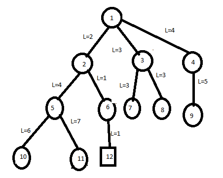
In this we will take node 1 as E node and generate the children of node 1 i.e. 2, 3, 4.
By using ranking function, we will select the next path with minimum cost of 2, 3, 4 nodes having cost 2,3,4 respectively. Selected node is node 2.
Now children of node 2 and its children are 5 and 6.
Select node 6. Now we will get the 12 which has minimum cost as 1.
- Let t be state space tree and c () becomes cost function for the nodes in t.
- If x is a node in t then c(x) is the minimum cost of any node in sub tree with root x.
- Hence c (t) becomes the cost of minimum cost answer node in t.
- The algorithm uses two functions as least_cost () and add_node().
- Least_node () finds a live node with least c () which is deleted from the list of live nodes and returned.
- Add_node() to delete and add live node from or to the list of live nodes.
- We are given n no. Of objects with weights Wi and profit Pi where I varies from 1 to n and also a knapsack with capacity M
- The problem is, we have to fill the bag with the help of n objects and the resulting profit has to be maximum.
- This problem is similar to ordinary knapsack problem but we may not take a function of an object.
Example:
Profit | 10 | 10 | 12 | 18 |
Weight | 2 | 4 | 6 | 9 |
In this problem we find upper bound and lower bound for each node.
- To calculate upper bound,
Place first item in knapsack calculate remaining weight ie. 15-2=13
Place next item in knapsack and remaining weight is 13-4=9
Place next item in knapsack and remaining weight is 9-6=3
Fraction is not allowed in calculation of upper bound in knapsack hence next item cannot placed in knapsack.
Profit=p1+p2+p3=10+10+12=32 ie. Upper bound
- To calculate lower bound,
Fraction is allowed in calculation of lower bound in knapsack hence next item can placed in knapsack.
Lower bound=10+10+12+(3/9*18)=32+6=38
Knapsack is maximization problem but branch and bound can be applied on minimization problem.
Hence to convert maximization problem into minimization we have to take negative sign for upper bound and lower bound.
Therefore upper bound (U)=-32
Lower bound(L)=-38
We choose the path which has minimized difference of upper bound and lower bound.
If the difference is equal then choose the path by comparing upper bound and discard node with maximize upper node.
Now calculate upper and lower bound for remaining nodes.
For node 2,
U=10+10+12=32 ≈ -32
L=10+10+12+(3/9*18)=32+6=38 ≈ -38
For node 3,
U=10+12=22
L=10+12+(5/9*18)=32 ≈ -32
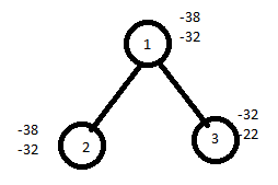
Calculate the difference of upper bound and lower bound for 2,3.
For node 2, U-L=-32+38=6
For node 3,U-L=-22+32=10
Select node 2 since it has minimum difference value of 6.
Similarly continues the process,
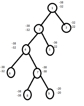
Calculate difference of lower and upper bound of nodes 8 ,9.
For node 8,U-L=-38+38=0
For node 9,U-L=-20+20=0
Here difference is same hence compare upper bound of node 8 and 9.
Discard the node with maximum upper bound.
Consider the path from 1 2478
The solution for 0/1 knapsack problem is (1,1,0,1)
Maximum profit= ∑PiXi=10*1+10*1+12*0+18*1=10+10+18=38
FIFO branch and bound solution
Let assume above example in this problem.
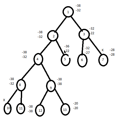
Initially node 1 is E node and queue of live nodes are empty.
Here U=-32 hence node 2 and 3 are generated as children of node 1 and added to the queue. The value of upper bound remain unchanged.
Now node 2 becomes E node and its children are added to the queue.
Next node 3 is expanded and its children are generated. Node 6 is also added to the queue. Node 7 is killed as L(7)>U.
Next node 4 is expanded. Continue the process until it get the solution.
Steps to solve travelling salesman problem:
Step 1: reduce given cost matrix in which every row and column is reduced. This can be done as follows:
Row Reduction:
- Take the minimum element from first row,subtract it from all elements of first row,next take minimum element from second row and subtract it from second row. Similarly apply the same procedure for all rows.
- Find the sum of element, which were subtracted from rows.
- Apply column reductions for the matrix obtained after row reduction.
Column reduction
- Take the minimum element from first column, subtract it from all elements of first column, next take minimum element from the second column and subtract it from second column. Similarly apply the same procedure for all columns.
- Find the sum of elements, which were subtracted from columns.
- Obtain the cumulative sum of row wise reduction and column wise reduction.
- Cumulative reduced sum=Row wise reduction sum + Column wise reduction sum.
- Associate the cumulative reduced sum to the starting state as lower bound and α as upper bound.
Step 2: Calculate the reduced cost matrix for every node.
If path (i,j) is considered then change all entries in row i and column j of A to α.
Set A(j,1) to α.
Apply row reduction and column reduction except for rows and columns containing only α. Let r is the total amount subtracted to reduce the matrix.
Find ĉ(S)= ĉ(R)+A(i,j)+r.
Repeat step 2 until all nodes are visited
Example:
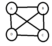
Given cost adjacency matrix
| A | B | C | D |
A | ∞ | 4 | 6 | 2 |
B | 7 | ∞ | 5 | 3 |
C | 2 | 1 | ∞ | 9 |
D | 8 | 7 | 2 | ∞ |
LET stating node is A
So upper bound= ∞
Row Reduction
∞ | 2 | 4 | 0 |
4 | ∞ | 2 | 0 |
1 | 0 | ∞ | 8 |
6 | 5 | 0 | ∞ |
1 | 0 | 0 | 0 |
 Minimum value
∞ | 4 | 6 | 2 | 2 |
7 | ∞ | 5 | 3 | 3 |
2 | 1 | ∞ | 9 | 1 |
8 | 7 | 2 | ∞ | 2 |
Minimum value
Minimum value of each row is 2,3,1,2 respt.
Total reduction=(2+3+1+2)+1=9
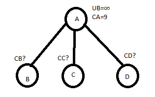
CA = 9
∞ | 2 | 4 | 0 |
3 | ∞ | 2 | 0 |
0 | 0 | ∞ | 8 |
5 | 5 | 0 | ∞ |
Let choose AB
So C[A,B] = 2
CA=9
PUT A ROW∞
B COLUMN∞
C[B,A] ∞
∞ | ∞ | ∞ | ∞ |
∞ | ∞ | 2 | 0 |
0 | ∞ | ∞ | 8 |
5 | ∞ | 0 | ∞ |
We get same column after row & column reduction. Therefore reduction=0
Hence, CB=C[A,B]+CA+REDUCTION
=2+9+0
=11
Let choose AB
C[A,C]=4 AND CA=9
PUT A ROW∞
C COLUMN∞
C[C,A] ∞
∞ | ∞ | ∞ | ∞ |
3 | ∞ | ∞ | 0 |
∞ | 0 | ∞ | 8 |
5 | 5 | ∞ | ∞ |
We get column after row & column reduction. Therefore reduction=5
∞ | ∞ | ∞ | ∞ |
3 | ∞ | ∞ | 0 |
∞ | 0 | ∞ | 8 |
0 | 0 | ∞ | ∞ |
So Cc=C[A,C]+CA+REDUCTION
=4+9+5=18
Lets choose AD
SO C[A,D]=0 & CA=9
PUT A ROW∞
D COLUMN∞
C[D,A] ∞
∞ | ∞ | ∞ | ∞ |
3 | ∞ | 2 | 0 |
0 | 0 | ∞ | 8 |
∞ | 5 | 0 | ∞ |
WE GET CAM AFTER row and column reduction as, reduction=2
∞ | ∞ | ∞ | ∞ |
1 | ∞ | 0 | ∞ |
0 | 0 | ∞ | ∞ |
∞ | 5 | 0 | ∞ |
So CD=C[A,D]+CA+REDUCTION=0+9+2=11
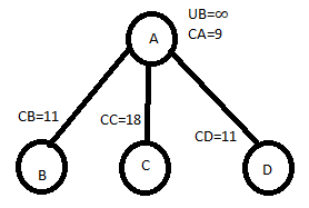
LETS CHOOSE AD
SO REDUCTION MATRIX IS,
∞ | ∞ | ∞ | ∞ |
1 | ∞ | 0 | ∞ |
0 | 0 | ∞ | ∞ |
∞ | 5 | 0 | ∞ |
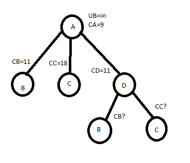
ENTERING NODE D.
LET CHOOSE ADB
C[D,B]=5 & CD=11
PUT D ROW∞
B COLUMN∞
C[B,D] ∞ & C[B,A] ∞
∞ | ∞ | ∞ | ∞ |
∞ | ∞ | 0 | ∞ |
0 | ∞ | ∞ | ∞ |
∞ | ∞ | ∞ | ∞ |
CAM AFTER REDUCTION IS SAME IE. REDUCTION=0
CB=5+11+0=16
LET CHOOSE ADC
C[D,C]=0 & CD=11
PUT D ROW∞
C COLUMN∞
C[C,D] ∞ & C[C,A] ∞
∞ | ∞ | ∞ | ∞ |
1 | ∞ | ∞ | ∞ |
∞ | 0 | ∞ | ∞ |
∞ | ∞ | ∞ | ∞ |
NOW REDUCTION = 1
∞ | ∞ | ∞ | ∞ |
0 | ∞ | ∞ | ∞ |
∞ | 0 | ∞ | ∞ |
∞ | ∞ | ∞ | ∞ |
CC=0+11+1=12
HENCE WE SELECT C, ADC
NOW WE EXPLORE NODE C
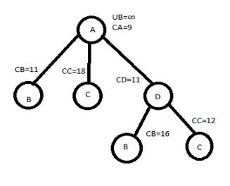
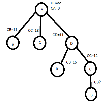
REDUCED MATRIX,
∞ | ∞ | ∞ | ∞ |
0 | ∞ | ∞ | ∞ |
∞ | 0 | ∞ | ∞ |
∞ | ∞ | ∞ | ∞ |
CHOOSE , ADCB
C[C,B]=0 & CC=0
PUT C ROW∞
B COLUMN∞
C[B,C] ∞ & C[C,A] ∞
∞ | ∞ | ∞ | ∞ |
∞ | ∞ | ∞ | ∞ |
∞ | ∞ | ∞ | ∞ |
∞ | ∞ | ∞ | ∞ |
NOW REDUCTION = 0
CB=0+12+0=12
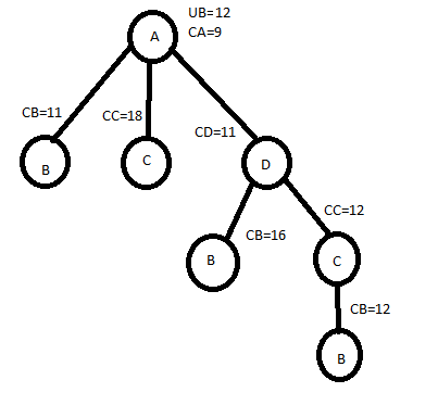
PATH IS, ADCBA WITH COST 12.