Unit - 4
2D Finite Element Analysis
The concept of Finite Element Analysis (FEA) basically includes fixing the spring equation, F = kδ, at a massive scale.
- There are numerous fundamental steps with inside the finite detail method:
- Discretize the shape into factors.
- These factors are linked to each other thru nodes.
- Determine a nearby stiffness matrix for every detail.
- Assemble a worldwide stiffness matrix for the general shape primarily based totally at the mixture of the nearby stiffness matrices.
- Build the carried out pressure vector.
- A 2D strong detail, be it aircraft pressure or aircraft strain, may be triangular, square or quadrilateral in form with immediately or curved edges. The most customarily used factors in engineering exercise are linear.
- Quadratic factors also are used for conditions that require excessive accuracy in strain, however they may be much less regularly used for sensible problems. Higher order factors have additionally been developed, however they may be much less regularly used besides for sure precise problems.
- The order of the 2D detail is decided via way of means of the order of the form features used. A linear detail makes use of linear form features, and consequently the rims of the detail are immediately.
- A quadratic detail makes use of quadratic form features, and their edges may be curved. The equal may be stated for factors of 0.33 order or higher. In a 2D version, the factors can most effective deform with inside the aircraft in which the version is defined, and in maximum conditions, that is the x-y aircraft. At any point, the variable, this is the displacement, has additives with inside the x and y directions, and so do the outside forces.
- For aircraft pressure problems, the thickness of the authentic shape is normally now no longer crucial, and is commonly handled as a unit amount uniformly all through the 2D version. However, for aircraft strain problems, the thickness is a crucial parameter for computing the stiffness matrix and stresses.
- Throughout this topic, it's far assumed that the factors have a uniform thickness of A. If the shape to be modelled has a various thickness, the shape desires to be divided into small factors, in which in every detail a uniform thickness may be used.
- On the opposite hand, components of 2D factors with various thicknesses also can be carried out easily, because the process is much like that of a uniform detail. Very few commercially to be had software program programs offer factors of various thickness.
Plane Stress-Strain, axi-symmetric problems in 2D elasticity
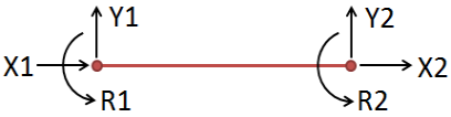
Line factors are related best at not unusual place nodes, forming framed or articulated systems together with trusses, frames, and grids.
Three-dimensional elasticity troubles are very tough to solve.
Thus we will first expand governing equations for -dimensional troubles, and could discover fundamental theories:
- Plane Strain
- Plane Stress
The fundamental theories of aircraft stress and aircraft strain constitute the fundamental aircraft trouble in elasticity. While those theories practice to significantly unique kinds of -dimensional bodies, their formulations yield very comparable area equations.
Since all actual elastic systems are three-dimensional, theories set forth right here could be approximate models. The nature and accuracy of the approximation will rely upon trouble and loading geometry.
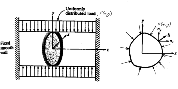
Consider an infinitely lengthy cylindrical (prismatic) frame as shown.
If the frame forces and tractions on lateral obstacles are impartial of the z-coordinate and don't have any z-component, then the deformation area may be taken in the decreased form
u = u(x,y), v= v(x, y), w = 0
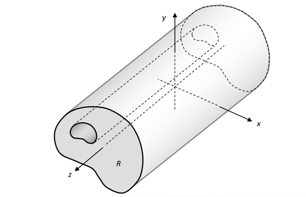
Consider a in which one dimension, egg. Alongside z, is small in assessment to the different dimensions with inside the problem.
Thru the thickness, and consequently they'll be about 0 for the duration of the whole domain. Finally, because the vicinity is skinny with inside the z direction it may be argued that the opposite non-0 stresses may have little version with z. Under those assumptions, the pressure discipline may be taken as:
The typical boundry conditions for plane stress problems in two dimensional analysos will be:
1. Loading may be pointed or ditributed over the plate
2. Supports may be fixed or roller


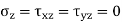
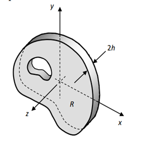
Fig: Distributed forces
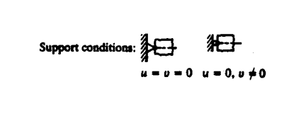
Fig: Support joints
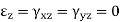
For isotropic materials and assuming

And γXZ = γYZ = 0
Yields

Where
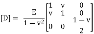
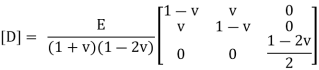
In the above equation D is the stress-strain matrix, E is the modulus of elasticity and v is the positions ratio
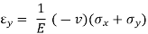
The strains in plane stress are given by:
{ε} = [C] {σ}
Or 
Where [C]-1 = [D]. Also
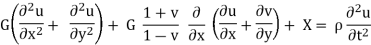
The basic partial equation for plane stress will be given as,
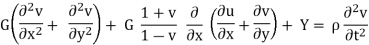
Where the shear modulus G is defined as

Plain Strain:
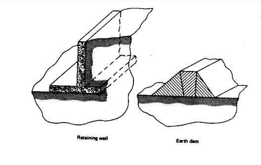
In this strain one deals with the situation in which direction of the structure in own direction, say it as z direction, it is very large compare with the dimensions of the structure in other two directions.
The geometry of the body is essentially that of a prismatic cylinder with one dimension much larger than others.
The applied forces act in xy plane, and do not vary in z direction. Some important applications of this representation occurs in the analysis of dams, tunnels, and other geotechnical works.
Typical loading and boundary conditions for plane strain problems in two-dimensional elasticity.
For isotropic materials and assuming
And τXZ = τYZ = 0
Yields

Where
With
σz = 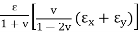
The basic partial differential equations for plane strain including body and inertia forces are

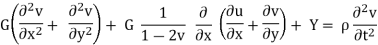
Where

Axisymmetric Problems:
Solids of revolution deforms symmetrically with respect to the axis of revolution.
Eg:
1. Cylinders subjected to internal and external pressures.
2. Rotating Circular Disks
Axisymmetric solids:
The solids which have axisymmetric loading, are module as axisymmetric solids. As seen from the figures below all stresses are independent of rotational angle.
Egg. Flywheel, bearing, thick-walled stress vessels
Conditions for axisymmetric problems:
1. The trouble area have to have an axis of symmetry.
2. The boundary conditions are symmetric approximately the axis. Therefore all BCs are unbiased of θ
3. All boundary conditions are symmetrical approximately
4. This condition usually satisfied for isotropic materials
5. Lastly, the solutions are unbiased of θ
Where there is symmetry in geometry and loads we can model such problems as special two-dimensional problems.
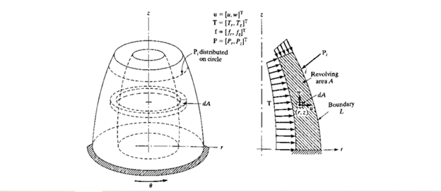
- Consider the fundamental quantity proven here.
- Here we observe that each one integrals are impartial of θ
- We can write strains for this case as
ε= [εr, εz, γrz, εθ]
- Using derivatives of displacements this can be written as
- The stress vector for this case is
σ = [σr , σz , τrz , σθ]
- Now the stress- strain relation is given as σ = D ε where D is
D = 
Axisymmetric for triangular elements:
The place of axisymmetric is now divided into triangular finite factors. By revolving those factors we really get the discretized stable object. Therefore eleven though every detail is a triangle, it really represents a stable ring of triangular section approximately the axis of symmetry.
- Following the discussion on CST and replacing x, y coordinates with r, z we have a similar formulation now. Using 3 shape function N1, N2 and N3 we write {u} = [N]{q} where
N = 
q = [q1, q2, q3, q4, q5, q6 ]T
Key Takeaways:
- Throughout this topic, it's far assumed that the factors have a uniform thickness of A. If the shape to be modelled has a various thickness, the shape desires to be divided into small factors, in which in every detail a uniform thickness may be used.
- The fundamental theories of aircraft stress and aircraft strain constitute the fundamental aircraft trouble in elasticity
- If the frame forces and tractions on lateral obstacles are impartial of the z-coordinate and don't have any z-component, then the deformation area may be taken in the decreased form
In numerical mathematics, the regular stress triangle detail, additionally referred to as the CST detail or T3 detail, is a form of detail utilized in finite detail evaluation that's used to offer an approximate answer in a 2D area to the precise answer of a given differential equation. The call of this detail displays how the partial derivatives of this detail's form feature are linear functions.
The detail offers an approximation for the precise answer of a partial differential equation that's parameterized bar centric coordinate system (mathematics)
The functions for the displacement in x and y direction can be defined as the above:
u(x, y) = a1 + a2 x + a3 y + a4 x2 + a5 xy + a6 y2+a7x3+ …
Here the’s are constants to be found from the boundary conditions on displacement. Notations for the three node triangle are shown in the figure below.

If we use best the linear phrases from the overall polynomial, the displacement characteristic is approximated by
u(x, y) = a1 + a2 x + a3 y
To examine the constants a1, a2, and a3, observe the displacement boundary situations which relate the non-stop displacement discipline u(x,y) to the unique displacements u1, u2, and u3 that arise on the nook nodes of the triangular element. (It isn't any any twist of fate that there are 3 unknown constants a and 3 unique node factor displacement boundary situations.) The nodes are numbered in a counter clockwise way as shown. These situations are:
u(x1, y1) = u1
u(x2, y2) = u2
u(x3, y3) = u3
Or
u1 = a1 + a2 x1 + a3 y1
u2 = a1 + a2 x2 + a3 y2
u3 = a1 + a2 x3 + a3 y3
3 Eqns. In 3 unknowns a1, a2, a3
Solve for a1, a2, a3 in terms of u1, u2, u3
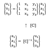
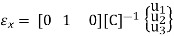
In the above, the matrix C contains the coordinates of the triangle corner nodes. Using C, the x direction displacement function is now expressed as:
u(x, y) = a1 + a2x + a3 y = [ 1 x y]  [1 x y] [C]-1
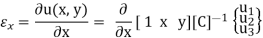
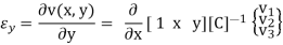
We may now find expressions for the extensional and shear strains within the element. The strain-displacement relations are given by
Using the displacement in the x coordinate to find the strain in x gives:
The development for displacement and strain in the y coordinate follows the same path as for the x coordinate. A linear displacement function is used as before.
v(x, y) = a4 + a5 x + a6 y
Applying the displacement boundary conditions to the y displacement function gives:
v(x1, y1) = v1 = a4 + a5x1 + a6 y1
v(x2, y2) = v2 = a4 + a5x2 + a6 y2
v(x3, y3) = v3 = a4 + a5x3 + a6 y3
Again , 3 Eqns. In 3 unknowns a4, a5, a6
Solve for a4, a5, a6 in terms of v1, v2, v3

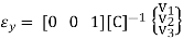
The linear strain in the y coordinate is given by the following.
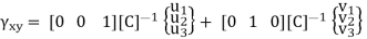
Using the u(x,y) and v(x,y) displacement functions, the shear strains within the element are given as:
Displacement additives are generally ordered so that each one of the displacements at a node are grouped collectively while defining the detail displacement vector d.
{d} = 
The matrix B(x,y) is then described so that it will specific the connection among the
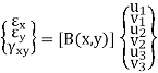
Lines with inside the detail and the detail node factor
(B is a consistent for the CST detail, however is proven right here as B(x,y) considering the fact that it is able to be a feature of x and y for different factors.) The detail stiffness matrix is given by
{k} = 
In which E is the pliancy matrix for the strain-stress country below consideration. For triangular factors utilized in planar problems, E can also additionally describe a country of aircraft strain, aircraft stress, or a case wherein the strain and stress country is symmetric with appreciate to a vital axis (axisymmetric case).
The matrix C may be inverted symbolically the usage of the coordinates of the triangle node factors as recognized quantities.
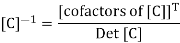
Det [C] = 1 (x2y3 – x3y2) – 1 (x1y3 – x3y1) + 1(x1y2 – x2y1) = 2A
Here A is the area of the triangle. The cofactors of C are given by:
Cof11 = x2y3 – x3y2 cof12 = – (y3 – y2) cof13 = (x3 – x2) etc.
Using the determinate and the cofactors as found above, the strain-node point displacement expression becomes:
In the above, all entries in B are constants because of the assumption on the degree of the displacement polynomial used for u(x,y) and v(x,y). For elements with higher order polynomials, B = B(x,y).
The element stiffness matrix can now be found using the integral relationship
{k} = 
Since B is a constant for this element, the above reduces to
[k] = [B]T [E][B]  [BCST]T[E][BCST]
 = [BCST]T[E] [BCST]At
The product BTEB can be computed and a closed form expression obtained for the constant strain triangle stiffness matrix.
Load Vector:
The load vector f consists of the outside nodal forces as targeted with inside the enter record and of the meeting of the detail masses. These detail masses may be subdivided into the subsequent components
1. Equivalent nodal forces because of thermal results, results as a consequence of distinction in attention and preliminary strains. Summing those results effects in an equal preliminary strain, which may be converted to nodal masses.
2. Equivalent nodal forces as a consequence of preliminary stresses.
3. Equivalent nodal forces as a consequence of masses on detail boundaries.
4. Equivalent nodal forces as a consequence of acceleration results (useless weight).
Equilibrium
Invoking the theory of the digital displacements, the equilibrium equations of the detail assemblage are
Ku = f Where the matrix K is the stiffness matrix of the element assemblage
And the vector f is the right hand side vector
With fg =   The contribution of the element body forces. ft =   The contribution of the element surface tractions. f ε0 =   The effect of the element initial strains. f σ0 =   The effect of the element initial stresses. fc
| (29.35) |

The contribution of the concentrated nodal forces.
Stress and reaction forces calculations for CST:
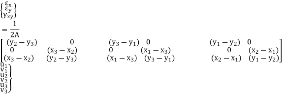
Quicken presently makes use of planar constraint stress triangle factors (CST). CST factors are the best planar factors to create, remedy and understand, and as such are perfectly suited to FEA on cell platforms. The essential issue of CST factors is that they may be overly stiff in bending, however, this will be addressed via way of means of growing the quantity of factors to your FEM till convergence is accomplished.
Initially the coarse version with best 10 factors indicates a y displacement of 0.251 that's an extended manner from specific answer of 1.031. However, as soon as the quantity of factors is improved to eight factors via the “beam” intensity, affordable displacement accuracy is accomplished to inside 5%. Sixteen factors via the intensity is inside 2%.
Key Takeaways:
- The detail offers an approximation for the precise answer of a partial differential equation that's parameterized bar centric coordinate system (mathematics)
- To examine the constants a1, a2, and a3, observe the displacement boundary situations which relate the non-stop displacement discipline u(x,y) to the unique displacements u1, u2, and u3 that arise on the nook nodes of the triangular element
- The development for displacement and strain in the y coordinate follows the same path as for the x coordinate. A linear displacement function is used as before.
After the calculation has been efficiently completed, the post-processor shows the calculation consequences graphically. Here, the statistics interpretation takes place. This includes, except the displacements, additionally stresses and nodal forces.
The displacements offer facts approximately the geometric deflections of the aspect. An immoderate visualization guarantees that even very small displacements may be seen. The scaling aspect may be selected individually. The equal strain permits to decide the mechanical sturdiness of the aspect.
These need to now no longer be more than the supportable most stresses. The maximum specific stresses are on the Gauss points, considering the fact that they may be calculated from the precise changes (distortions) of the person factors. All different stresses, with inside the factors or with inside the nodes, end result from averaged Gauss factor stresses and their validity isn't that accurate. The help reactions may be examine out from the nodal forces.
This may be of hobby for the similarly layout of additives of connecting parts, considering the fact that an aspect not often seems alone. The distortions in all 3 coordinate directions, absolutely the price of distortions, the stresses according to element, with inside the nodes of the factors and with inside the Gaussian nodes, may be displayed.
Also the ensuing nodal forces may be visualized direction-dependent. For the thermos-mechanical evaluation moreover the temperature, the thermal strain, the thermal forces and the warmth glide are to be had as well.
The non-linear and herbal frequency evaluation ties this to the respective load or frequency. The shape may be displayed deformed, non-deformed or overlapped. A self-described filtering of the show statistics is likewise feasible with the intention to spotlight precise areas.
Procedure:
- The post processing technique is likewise crucial so one can beautify the uncooked end result acquired from the processing reaction after the convolution manner is achieved among the authentic photograph and the gray-stage template at one of a kind orientations.
- The linearization manner gives a binary map of values that lets in for a higher visualization of vessels and heritage from the end result photograph.
- However, because of excessive noise degrees with inside the authentic photograph, a few entropy values stay after the linearization manner, which need to be eliminated so one can have a more suitable very last photograph end result.
- After the reaction photos had been acquired, a post processing technique turned into implemented to them so one can gain an more suitable presentation of the results, leaving simplest the ones pixels belonging to blood vessels and doing away with the relaxation of the records with inside the photograph, that's taken into consideration as heritage or noise.
Special tricks and interpretation of results:
When the SOLIDWORKS Simulation solver is whole, the effects are routinely loaded into the effects folder. Typically, the effects folder will consist of default plots of von Misses strain, displacement and strain (in that order) and after the run is whole the von Misses strain plot could be highlighted and routinely display at the screen.
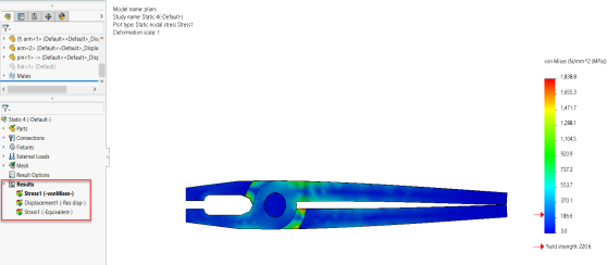
Figure: Typical von Mises stress result plot that displays after solution is complete
Since the aim of many simulations is to evaluate whether or not and wherein the component will fail, the temptation is to begin diving into the strain effects without delay. I strongly endorse towards this. Instead, double click on at the displacement plot and start put up processing through very well interrogating the deflection and deformation of your component/meeting.
The first aspect we frequently study from the displacement plot is that there may be something incorrect with our evaluation. Sometimes the strain effects appearance OK, however the displacement plot will display deflections of lots or maybe hundreds of thousands of inches or mm! When this happens, we understand without delay that something is incorrect with our setup.
Typically, the component/meeting isn't fixture correctly, or we've got now no longer setup our interactions correctly, and consequently the effects are garbage. In FEA parlance, we've got did not restrain all 6 inflexible frame modes. In this situation there may be no want to continue similarly with put up processing; we need to pass again to the setup, perceive and connect the problem and re-run the evaluation.
If we by skip the deformation sanity check, the subsequent aspect I endorse is to set the deformed form scale appropriately. In maximum static simulations, deflections are small relative to the geometry we're analyzing (in reality small deflections are a pre-considered necessary for a legitimate linear static evaluation).
Small deflections are frequently slightly seen to the bare eye, making it difficult to visualize wherein our component/meeting is bending and deflecting. To spotlight relative deflections, SOLIDWORKS Simulation can increase the significance of the deformation through making use of a scaling issue.
Exaggerated deformations are the default plotting option, so be careful; I’ve frequently heard clients whine that the effects don’t appearance proper due to the fact the component turned into bending so much.
Remember that the exaggerated deformed form is only a visible resource to assist us perceive regions of exceedingly huge deformation. Sometimes a huge deformation scale can lead us astray. For example, in my plier evaluation if we follow the automated deformed form scale (2.ninety eight instances exaggeration) the arms of the pliers will by skip via every other that is glaringly now no longer possible.
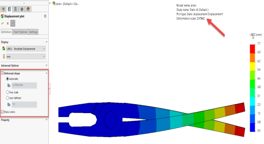
Figure: Strange looking results with Automatic deformed shape scale factor
In this specific case, I’d need to set the deformed form scale issue to “True scale”, which indicates the recommendations of the handles contacting each other correctly.
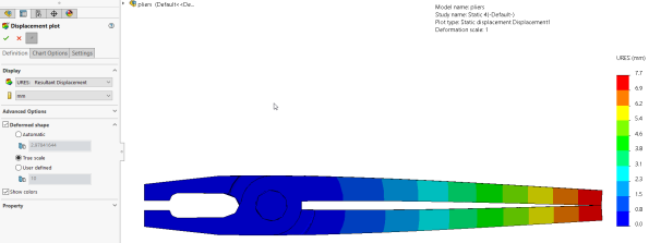
Figure: Expected results with True scale factor applied
The subsequent step is to animate the displacement plot. Right click on at the displacement plot with inside the effects folder and choosing animate.
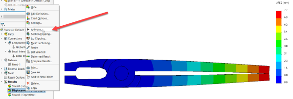
Figure: How to animate your displacement plot
Once the animation assets supervisor displays, hit the play button and examine how your version deforms and deflects beneath the implemented loads, furnishings and interactions. Most designers and engineers have a terrific instinct for the way their components and assemblies will deform. A displacement animation is a beneficial manner to verify that your instincts are correct (or possibly now no longer).
2. Use “Discrete” instead of “Continuous” for contour plots
When reading your pressure or deformation outcomes keep in mind switching the contour show from “Continuous” to “Discrete”. Right click on over the legend after which select “Fringe Options” after which “Discrete”.
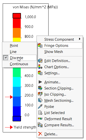
Figure: How to switch from “Continuous” to “Discrete” contour display’
“Continuous” will blend and blur together the colors in the legend as shown in the image below.
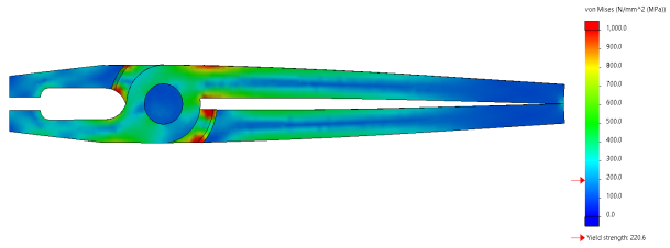
Figure: “Continuous” von Mises stress
Whether to use “Discrete” or “Continuous” is a non-public preference, however I discover the discrete alternative higher for put up processing contour plots.

Figure: “Discrete” von Mises stress
3: Reset both the upper and lower bounds of your legend
When plotting pressure outcomes, the default top restrict proven at the legend could be the most pressure for your version.
The most pressure with inside the version is mostly a local “warm spot” related to a fixture or location of excessive touch pressure. This will frequently go away a “sea of blue” with inside the relaxation of the version indicating stresses which are low relative to the most with inside the version, as validated with inside the photograph under.
However, the blue and inexperienced colorations may also really be excessive stresses relative to the electricity of the material.
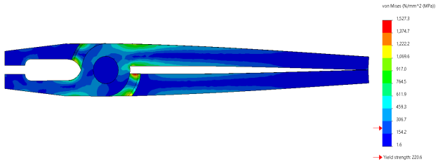
Figure: Default upper and lower bounds for von Mises stress
We understand that stresses close to furnishings aren't correct and have to be taken into consideration with skepticism or ignored.
So why set the top sure of the color legend at the most (probably inaccurate) pressure end result close to a fixture or warm spot? Instead, test with adjusting the top and decrease bounds for greater perception into the stresses for your version and to take away the “sea of blue”.
Left click on at the top or decrease sure variety of your legend and key in exceptional numbers. In the instance under I selected 500 MPa as my top restrict. I additionally modified the decrease restrict from the default 1.6 MPa to zero MPa.
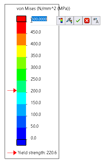
Figure: Changing the upper bound of von Mises stress
These adjustments create spherical variety increments of precisely 50 MPa for every color band. If I had left the decrease sure at 1.6 MPa, this will now no longer had been within side the case, as it divides the color bands lightly among top and decrease bounds. Having the decrease sure be precisely zero MPa makes logical sense. Note that within side the photograph under we now see tons greater orange, yellow and inexperienced which might be regions of excessive pressure, a long way in extra of the yield electricity of the material, indicating that a layout extrude is important in this version. This changed into much less apparent with the default bounds at the pressure plots.
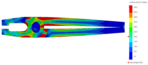
Figure: Modified upper and lower bounds for von Mises stress
There are plenty of different beneficial hints for put up processing in SOLIDWORKS Simulation however I desire those suggestions could be beneficial and enhance your information of the outcomes. Now pass layout a few modern merchandise with the assist of SOLIDWORKS Simulation.
CAE Reports:
- Finite Element Analysis (FEA) has been, for lots decades, the area of excessive tech engineers, PhD’s and specialists. Scientists in labs huddled over mainframe servers past due at night, writing and re-writing simulations that required the committed time of effective laptop servers.
- Due to this characterization of the method, till the 1990’s, FEA evaluation become restrained nearly absolutely to the aeronautics, automotive, protection and nuclear industries.
- It became certain incredibly of a ‘darkish art’ with recognize to the greater traditional production and layout surroundings of CAD/CAM.
- The equipment are a lot greater reachable and less complicated to examine that it's far not tucked away inner studies centers or housed on large servers.
- FEA is a laptop-primarily based totally method used for modeling complicated merchandise and systems.
- These simulations arise in a digital surroundings for the motive of ‘solving’ or locating a sequence of answers to doubtlessly complicated overall performance issues.
- It is beneficial for all tiers of technology and engineering disciplines. Specifically, as carried out to cloth sciences and engineering, it's far used to calculate the power and behavioral traits of a fabric below situations including strain, vibration and deflection.
- It may be used to research big-scale and small-scale behaviors of materials. FEA software program is now quicker and less complicated to apply than ever earlier than. It is not to be had from only some businesses and springs in a whole lot of tiers of complexity.
- It is now so various that it could be unfold round production centers or even embedded into different layout and manage software program this is already being utilized by operators. FEA works via way of means of breaking down a big shape, with excessive tiers of bodily complexities and mathematical discontinuities, into smaller, greater possible sections.
- Each segment represents the cloth homes of its nearby area. By reducing the shape into smaller and smaller sections, the simulator profits an information of the way the bigger shape will reply to outside or inner stimuli.
- The begin of this method starts via way of means of figuring out the location of a theoretical array of ‘nodes’ at the shape.
- The NODE is an unmarried factor in the 2D or 3-d shape. Each node is programmed with the cloth and structural information of it’s on the spot place.
- The addition of traces among the nodes creates a MESH shape. The meshing encloses smaller, less difficult sections of the total component. The denser the mesh, the greater particular the effects could be for the total machine, however the greater complicated the computations.
- The areas which might be enclosed via way of means of the mesh shape are a set of finite ELEMENTS, hence, Finite Element Analysis.
- Each detail is described via way of means of the greater easy equations regarding strain, force, inertia, thickness, power, acceleration, temperature, etc. concerning the border situations alongside that precise mesh and people situations in the detail.
- The laptop software program maintains a list of the person elements, their neighboring elements, and the inner and border situations.
- All of the mesh equations in the machine are solved concurrently and the effects are used to decide how every node responds while outside stimulus is carried out to it, or to its neighboring elements.
- When a simulation application is accomplished and stressors are carried out to the machine, every detail starts to regulate its equations. These changes will both relieve or create extra stresses during the mesh, converting border situations for its buddies, simply as its buddies will alternate its personal border situations.
- If the nodes and meshes had been programmed properly, the machine will ultimately paintings all of the stresses out of the equations and start to settle. This is called “convergence” and an answer is created. The laptop then applies this option to every person node and from this, receives a theoretical strain and deflection characteristic for every segment of the shape.
- This end result may be analyzed graphically or numerically in the application software program. The answer is in comparison to the tolerances of the machine to decide if the shape is robust sufficient for the application, even earlier than the component is manufactured.
- Programming the place of the person nodes is vital. The nodes may be programmed with any quantity of density. This density is what defines the precision of the reaction of the nearby region. Regions of better node density will go back a greater correct end result for that region.
- However, the greater nodes in a region, the greater computations that should take location to get a converging end result, extending the run-time and reminiscence utilization of the machine. It is sensible to application an excessive density of nodes best in areas receiving big quantities of strain or different vital factors of interest, whilst preserving a minimal quantity of nodes during the majority cloth so that it will see much less complicated stressors.
- By including and subtracting nodes in key areas, the operator also can help the laptop in reaching convergence.
Key Takeaways:
- The scaling aspect may be selected individually. The equal strain permits to decide the mechanical sturdiness of the aspect.
- All different stresses, with inside the factors or with inside the nodes, end result from averaged Gauss factor stresses and their validity isn't that accurate. The help reactions may be examine out from the nodal forces.
- The linearization manner gives a binary map of values that lets in for a higher visualization of vessels and heritage from the end result photograph.
- Typically, the effects folder will consist of default plots of von Misses strain, displacement and strain (in that order) and after the run is whole the von Misses strain plot could be highlighted and routinely display at the screen.
- In FEA parlance, we've got did not restrain all 6 inflexible frame modes. In this situation there may be no want to continue similarly with put up processing; we need to pass again to the setup, perceive and connect the problem and re-run the evaluation.
References:
1. K. J. Bathe, Finite Element Procedure, Prentice-Hall of India (P) Ltd., New Delhi, 1996.
2. Cook R. D., Finite Element Modeling for Stress Analysis, John Wiley and Sons Inc, 1995.
3. G.R. Liu S. S. Quek, The Finite Element Method- A Practical Course, Butterworth Heinemann, 2013.
4. Fagan M. J., Finite Element Analysis Theory and Practice, Harlow Pearson/Prentice Hall, 2012.
5. S. Moaveni, Finite element analysis, theory and application with Ansys, Pearson, Third Edition, 2011.
6. David V. Hutton, Fundamental of Finite Element Analysis, Tata McGraw-Hill, 2017.


