Unit - 5

Non-Linear and Dynamic Analysis

5.1 Nonlinear analysis: Introduction to nonlinear problems, comparison of linear and nonlinear analysis, types of nonlinearities, stress-strain measures for nonlinear analysis, analysis of geometric

Introduction:

• The principal purpose is that reaction spectrum evaluation relies upon on superposition, which does now no longer practice for nonlinear behavior. It is vital to apply step by step integration, additionally referred to as time records or reaction records evaluation.
• For linear evaluation all structural additives are elastic, and most effective elastic residences are wished for evaluation. For nonlinear evaluation, a few additives can yield, and extra inelastic residences are wished for those additives.
• These residences are extra complex than the elastic residences. In linear evaluation, the forces with inside the structural additives are computed, and the overall performance is classified the usage of energy demand/capacity (D/C) ratios.
• In nonlinear evaluation, inelastic deformations as additionally calculated, and the overall performance is classified the usage of and each deformation and energy D/C ratios. An instance of an inelastic deformation is the rotation at a plastic hinge.
• Formulas for energy capacities were advanced and delicate over a protracted length of time, and are properly understood.
• Formulas for deformation capacities are extra recent, much less delicate, and much less properly understood. A linear evaluation version generally calls for just a few aspect kinds (bar, beam, column, shell).
• For a nonlinear version the selection of aspect kinds is larger, due to the fact there are numerous exceptional styles of nonlinear behavior. For elastic additives the critical residences are elastic stiffness’s which include EI and EA, which might be normally easy and pretty properly standardized.
• For inelastic additives the critical residences consist of things like yield energy, post-yield behavior, and stiffness’s degradation below cyclic loading, further to the preliminary elastic stiffness.
• Inelastic (nonlinear) modeling is extra complicated than elastic (linear) modeling. It calls for extra judgment and a deeper know-how of structural behavior. Nonlinear evaluation calls for an awful lot extra pc time.

Nonlinear Analysis:

• In arithmetic and technological know-how, a nonlinear device is a device wherein the extrude of the output isn't proportional to the extrude of the enter.
• Nonlinear troubles are of hobby to engineers, biologists, physicists, mathematicians, and plenty of different scientists due to the fact maximum structures are inherently nonlinear in nature. 
• Nonlinear dynamical structures, describing adjustments in variables over time, may also seem chaotic, unpredictable, or counterintuitive, contrasting with an awful lot easier linear structures.
• Typically, the conduct of a nonlinear device is defined in arithmetic through a nonlinear device of equations, that is a hard and fast of simultaneous equations wherein the unknowns (or the unknown features with inside the case of differential equations) seem as variables of a polynomial of diploma better than one or with inside the argument of a feature which isn't a polynomial of diploma
• In different words, in a nonlinear device of equations, the equation(s) to be solved can't be written as a linear aggregate of the unknown variables or features that seem in them.
• In particular, a differential equation is linear if it's far linear in phrases of the unknown feature and its derivatives, despite the fact that nonlinear in phrases of the opposite variables acting in it.
• As nonlinear dynamical equations are hard to solve, nonlinear structures are typically approximated through linear equations (linearization). This works properly as much as a few accuracy and a few variety for the enter values, however a few exciting phenomena together with solutions, chaos, and singularities are hidden through linearization. It follows that a few factors of the dynamic conduct of a nonlinear device can look like counterintuitive, unpredictable or maybe chaotic.
• Although such chaotic conduct may also resemble random conduct, it's far in reality now no longer random.
• For example, a few factors of the climate are visible to be chaotic, wherein easy adjustments in a single a part of the device produce complicated results throughout.
• This nonlinearity is one of the motives why correct long-time period forecasts are not possible with modern technology. Some authors use the time period nonlinear technological know-how for the take a look at of nonlinear structures. This time period is disputed through others:

Physical nonlinearities with inside the mechanical conduct of systems can be categorized in extraordinary groups:

• Large deformations, probably main to huge strains
• Instabilities together with snap-thru or bifurcation buckling of slim beams or skinny shells
• Non-linear cloth conduct, e.g., huge-stress deformation of rubber or yielding of metals
• Changing touch conditions an instance trouble inclusive of all 3 abovementioned kinds of non-linearity is the simulation of leveling of skinny steel strips. Treating non-linear structures numerically is costly. Most of the time, answers can handiest be carried out with the aid of using dividing the loading records into many small increments.

Choosing the incorrect evaluation method can save you the detection of risky buckling phenomena. CAE Simulation & Solutions has accumulated large revel in in treating complicated nonlinear troubles with the Finite Element Method.

Nonlinear evaluation

A nonlinear evaluation is an evaluation in which a nonlinear relation holds among carried out forces and displacements. Nonlinear results can originate from geometrical nonlinearity’s (i.e. big deformations), fabric nonlinearity’s (i.e. elasto-plastic fabric), and contact.

These results bring about a stiffness matrix which isn't consistent throughout the weight application. This is against the linear static evaluation, in which the stiffness matrix remained consistent.

As a result, a distinct fixing approach is needed for the nonlinear evaluation and consequently a distinct solver. Modern evaluation software program makes it viable to gain answers to nonlinear problems.

However, skilled talent is needed to decide their validity and those analyses can without problems be inappropriate. Care ought to be taken to specify suitable version and answer parameters.

Understanding the problem, the position performed through those parameters and a deliberate and logical technique will do a lot to make certain a a success answer. The supply of this nonlinearity may be attributed to a couple of device properties, for example, materials, geometry, nonlinear loading and constraints.

Geometric Nonlinearity

In analyses regarding geometric nonlinearity, modifications in geometry because the shape deforms are taken into consideration in formulating the constitutive and equilibrium equations. Many engineering programs inclusive of metallic forming, tire evaluation, and clinical tool evaluation require using big deformation evaluation primarily based totally on geometric nonlinearity.

Small deformation evaluation primarily based totally on geometric nonlinearity is needed for a few programs, like evaluation regarding cables, arches and shells.

Material Nonlinearity

Examples of nonlinear fabric fashions are big strain (viscos) elastic-plasticity and hyper elasticity (rubber and plastic materials).

Constraint and Contact Nonlinearity

Constraint nonlinearity in a device can arise if kinematic constraints are gift with inside the version. The kinematic degrees-of-freedom of a version may be confined through enforcing regulations on its movement.

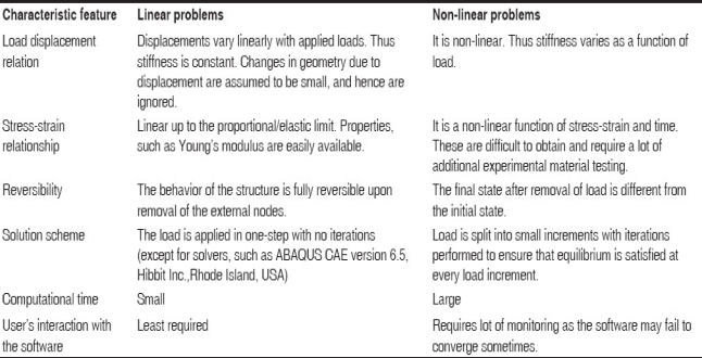
Comparison between linear and nonlinear analysis:

Types of Nonlinearities:

The Non-Linearity in any finite detail evaluation might be of the subsequent type:

Contact Non linearity:

Contact definition and operating is complex. The touch and goal surfaces must be described with due consideration. During evaluation, because of deformation the 2 surfaces can alternate orientation that's in which the touch and goal surfaces help. The touch nodes/floor will then detect/look for goal floor. Assigning right stiffness to the touch factors is likewise necessary.

Example for that is metallic elimination technique simulation. While machining the device gets rid of the metallic in shape of chips, to be able to simulate this detail start and rot must be modeled. Another instance is blade rub with case or lack of positive part of blade in case of turbine and its interplay with the turbine casing. Modelling and simulation of such eventualities must recollect the converting boundary conditions.

Material Non linearity:

The converting stiffness of the cloth because of performing hundreds introduces non-linearity with inside the system. The converting stiffness because of various temperatures influences the evaluation. Typical cloth behaviors - Creep, Plasticity, Elastic-plastic conduct, Hardening etc. represent demanding situations in linear evaluation. Good manner to recognize that is thinking about ductile or brittle fracture.

For a brittle cloth there may be no plastic deformation earlier than fracture (cleavage fracture) while for ductile cloth is preceded via way of means of necking and has considerable plastic deformation(cup and cone sort of fracture). So for ductile cloth the crack propagation takes place for positive length after initiation.

To examine this, most effective giving linear cloth residences isn't always sufficient (linear stress-pressure curve), elastic-plastic residences are needed. Other instance might be modelling residual compressive stresses with inside the version to simulate shot-peening.

Geometric Non Linearity:

This is the non-linearity going on because of huge deformation, huge pressure, Stress stiffening and softening.

Whenever we've huge deformation the linear pressure conduct wishes to be corrected with the inflexible frame movement and deformation. Certain examples for this may be: Modal evaluation for rotating additives. Rotating additives inclusive of turbine blades are subjected to centrifugal hundreds which bring about alternate in stiffness.

This adjustments the frequencies to positive extent (Fundamental Eigen frequency of a Rotating Blade). So modelling/assessment has to account for such adjustments. One not unusual place instance is buckling of narrow additives, positive narrow stress vessels have buckling tendency which must be taken into consideration for predicting the deformation in them other than the operational hundreds. This deformation wishes to deliver to the small lines going on at the frame.

Stress strain analysis:

Thus, the Cauchy strain that's primarily based totally at the modern-day configuration of the shape comes into play. However, it isn't immediately viable to apply this strain with inside the finite detail equations as defined with inside the segment four of this article. Hence, different strain and stress measures along with the 2d Piola Kirchhoff strain and the Green Lagrangian stress tensor come into existence.

Emphasis is laid best at the 2d Piola Kirchhoff strain tensor and the Green Lagrangian stress tensor, eleven though there are different strain and stress measures which can be in use in business software’s.

I actually have tried to logically divide the contents of this article, with: Section 2 explaining the simple trouble in a geometrical non-linear finite detail analysis Section three explaining the precept of digital displacements with an inexpensive background Section four describes in element the problem in making use of the precept of digital displacements the usage of the Cauchy strain Section five defines different strain and stress measures: 2d Piola Kirchhoff strain and the Green Lagrangian stress I actually have tried to result in the bodily interpretation of the 2d Piola Kirchhoff strain and the Cauchy strain in segment 6.

Body undergoing large displacements, large rotations, large strains

For a geometric non-linear analysis, we begin first with the continuous mechanics formulation considering the body being subjected to;

• Large displacements
• Large rotations
• Large strains

The configurations of the body at time t=0, time ‘t’ and at time t+Δt are shown below;

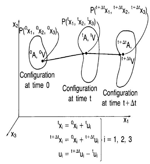
Figure: Configuration of the body at time t=0, time‘t’ and at time t+Δt

As stated earlier, the body during its deformation from time 0 to time ‘t’ and from time ‘t’ to time ‘t+Δt’ has undergone large displacements, large rotations and large strains.

It is probably profitable at this factor to encompass a be aware to explain the notations which have been used with inside the above figure.

A hard factor with inside the presentation of continuum mechanics relation for widespread big deformation evaluation is using powerful notation due to the fact there are numerous exclusive portions that want to be dealt with. In the above figure, the movement of the frame is taken into consideration in a fixed (stationary) Cartesian coordinate system.

All the static and kinematic variables are measured on this coordinate system. The coordinates of a standard factor P with inside the frame at time zero are zero^x, zero^x0^x; at time t, they're t^x, t^xt^x; and at time t+Δt they're t+Δt^x, t+Δt^xt+Δt^x, wherein the left superscripts talk over with the configuration of the frame and the subscripts are the coordinate axis (x, y, z correspond to 1,2,three). The notation for the displacements of the frame is much like the notation for the coordinates: at time t the displacements are tu, i=1,2,three and at time t+Δt the displacements are t+Δt^u, i=1,2,three. Therefore, we have;

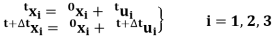
The increments in the displacements from time t to t+Δt are denoted by;

During the motion of the body, its volume, surface area and mass density, stresses and strains are changing continuously. The specific mass, area and volume of the body at times 0, t and t+Δt are denoted as: 0^ρ, t^ρ, t+Δt^ρ; 0^A, t+Δt^A; and 0^V, t^V, t+Δt^V, respectively.

Analysis of geometric nonlinearity:

• Large deflections or rotations.
• “Snap through.”
• Initial stresses or load stiffening.

For example, consider a cantilever beam loaded vertically at the tip.

If the end deflection is small, the evaluation may be taken into consideration as being about linear. However, if the end deflections are big, the form of the shape and, hence, its stiffness adjustments.

In addition, if the burden does now no longer stay perpendicular to the beam, the movement of the burden at the shape adjustments significantly.

As the cantilever beam deflects, the burden may be resolved right into an element perpendicular to the beam and an element performing alongside the duration of the beam.

Both of those outcomes make a contribution to the nonlinear reaction of the cantilever beam (i.e., the converting of the beam's stiffness because the load it consists of increases).

One might assume big deflections and rotations to have a sizable impact at the manner that systems convey loads. However, displacements do now no longer always should be big relative to the size of the shape for geometric nonlinearity to be important.

Consider the “snap through” below carried out strain of a big panel with a shallow curve, as proven in Figure.

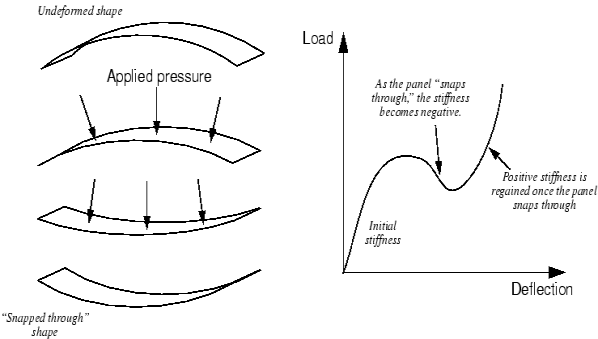
Figure. Snap-through of a large shallow panel

As the panel “snaps through,” the stiffness turns into negative. Thus, despite the fact that the importance of the displacements, relative to the panel's dimensions, is pretty small, there may be good sized geometric nonlinearity with inside the simulation, which need to be taken into consideration.

A crucial distinction among the evaluation merchandise have to be mentioned here: through default, Abacus/Standard assumes small deformations, at the same time as Abacus/Explicit assumes big deformations.

Key Takeaways:

• Nonlinear dynamical structures, describing adjustments in variables over time, may also seem chaotic, unpredictable, or counterintuitive, contrasting with an awful lot easier linear structures.
• Although such chaotic conduct may also resemble random conduct, it's far in reality now no longer random.
• A nonlinear evaluation is an evaluation in which a nonlinear relation holds among carried out forces and displacements.
• Examples of nonlinear fabric fashions are big strain (viscos) elastic-plasticity and hyper elasticity

5.2 Material nonlinearity, solution techniques for nonlinear analysis, newton Raphson method, Essential steps in nonlinear analysis

Material Non linearity:

The converting stiffness of the cloth because of performing hundreds introduces non-linearity with inside the system. The converting stiffness because of various temperatures influences the evaluation. Typical cloth behaviors - Creep, Plasticity, Elastic-plastic conduct, Hardening etc. represent demanding situations in linear evaluation. Good manner to recognize that is thinking about ductile or brittle fracture.

For a brittle cloth there may be no plastic deformation earlier than fracture (cleavage fracture) while for ductile cloth is preceded via way of means of necking and has considerable plastic deformation(cup and cone sort of fracture). So for ductile cloth the crack propagation takes place for positive length after initiation.

• The subsequent trouble is fabric nonlinearity; that is wherein the constitutive conduct of a fabric has a nonlinear pressure–displacement and stress–pressure response.
• The pressure in an artery wall can be upward of 25%, violating the belief that deformations are so small that adjustments of geometry may be neglected, and arterial tissue has a famous nonlinear stress–pressure response.
• This nonlinearity is addressed thru the usage of a hyperplastic constitutive model. Hyperplastic fashions are a feature of the deformation gradient tensor; the essential degree of fabric deformation and the pressure electricity densities from which they may be derived allow thermodynamically strong nonlinear stress–pressure conduct.
• Additionally, they may be insensitive to huge inflexible frame rotations and translations making them very appropriate for simulations wherein there's additionally geometric nonlinearity.

Solution Techniques:

The nonlinear load-displacement curve for a structure is shown in Figure.

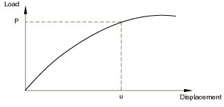
Figure. Nonlinear load-displacement curve

The goal of the evaluation is to decide this response. In a nonlinear evaluation the answer cannot be calculated via way of means of fixing an unmarried machine of linear equations, as might be completed in a linear problem.

Instead, the answer is observed via way of means of specifying the loading as a characteristic of time and incrementing time to acquire the nonlinear response. Therefore, Abacus/Standard breaks the simulation into some of time increments and unearths the approximate equilibrium configuration on the quilt of whenever increment.

Using the Newton method, it frequently takes Abacus/Standard numerous iterations to decide an appropriate method to whenever increment.

The time records for a simulation includes one or extra steps. You outline the steps, which commonly include an evaluation procedure, loading, and output requests. Different hundreds, boundary conditions, evaluation procedures, and output requests may be utilized in every step.

For example:

Step 1: Hold a plate among inflexible jaws.

Step 2: Add hundreds to deform the plate.

Step 3: Find the herbal frequencies of the deformed plate.

An increment is a part of a step. In nonlinear analyses every step is damaged into increments in order that the nonlinear answer course may be followed. You recommend the scale of the primary increment, and Abacus/Standard routinely chooses the scale of the following increments.

At the quilt of every increment the shape is in (approximate) equilibrium and outcomes are to be had for writing to the restart, data, outcomes, or output database files.

A generation is a try at locating an equilibrium answer in an increment. If the version isn't in equilibrium on the quilt of the generation, Abacus/Standard attempts any other generation. With each generation the answer that Abacus/Standard obtains ought to be toward equilibrium; however, every so often the generation technique might also additionally diverge—next iterations might also additionally pass far from the equilibrium state. In that case Abacus/Standard might also additionally terminate the generation technique and try to discover a answer with a smaller increment size.

Newton – Raphson Method:

As we understand that, linear equations does now no longer offers the reaction for nonlinear analysis. However, iterative collection of linear approximations with corrections may be used to examine the nonlinear shape. This iterative method of equilibrium generation referred to as Newton Raphson Method.

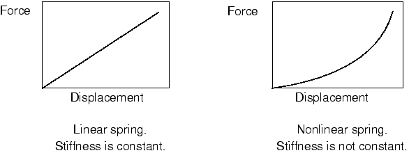
In case of nonlinear simulation, the stiffness of the shape isn't regular with recognize to loading (pressure as opposed to displacement plot isn't as immediately line).

This adjustments in stiffness are especially because of nonlinear fabric (fabric does no obeys hooks law, fabric plastically deform after elastic limit), nonlinear geometry (big deformation due small or large hundreds) or Contact nonlinearity (touch repute adjustments abruptly).

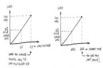
In such nonlinear scenarios, surprising adjustments in any aspects (like entire load software in unmarried step) might also additionally motive convergence difficulties. And therefore the hundreds are want to use regularly to keep away from convergence issues.

Let’s discuss through simple example as shown in graph.

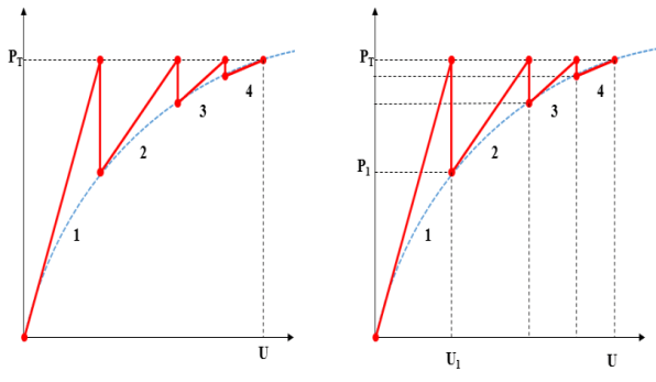
Figure: Newton Raphson Method

Figure suggests the curve (in blue color) constitute forces vs. Displacement relationship, right here vertical axis suggests the forces even as horizontal axis suggests the displacement. Newton Raphson approach is iterative process, however how does it carry out the iterations? In this approach the full load is carried out in first new release.

Equilibrium, however if P1≠ U1, then it outcomes is non equilibrium condition, for this reason similarly it break up the full pressure (slope of dotted line) and calculate new stiffness matrixes till equilibrium isn't carried out likewise it carry out the new release 1, 2, 3 & four after which equate with inner forces (P1, P2, P3 & PT) for that reason whilst the inner pressure fits with overall carried out forces, equilibrium is carried out and answer is stated to be converge. Here the distinction of PT – P1 is residual forces (out of balance). So it's miles essential to have smaller residual pressure in order that answer will converge. Let’s speak similarly with under example:

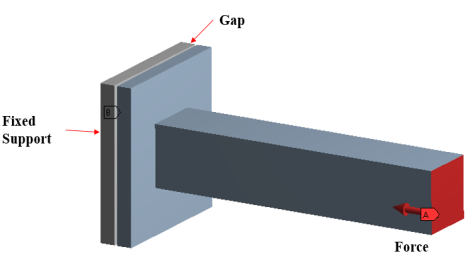
Figure suggests the 2 square plate, one plate is constant in all doff and different plate is hooked up to horizontal beam wherein the pressure is carried out. This horizontal pressure at the beam will purpose the plate to transport proper facet and get in touch with different plate & hence touch will hooked up and answer begin converging. Here the assignment is that, you want to set up nonlinear touch among the plates however whilst you follow complete pressure in unmarried step, it's going to effects in non-convergence issue

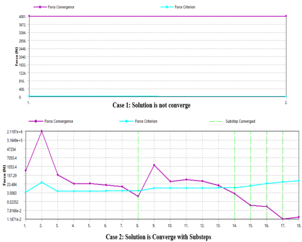
Figure: Solution Convergence Plot

Refer determine 3, case-1 suggests now no longer convergence (that is because of load carried out in unmarried step) and refer case-2, wherein load is carried out in special load steps ensuing pressure convergence meets the pressure criteria (Internal pressure). So as opposed to making use of load in unmarried load steps, in case you follow load step by step will assist to acquire the convergence.

Newton Raphson Method Convergence Techniques:

As mentioned above Newton Raphson acquire the convergence, however the reality is it does now no longer acquire in all of the cases. It will acquire best if the beginning configuration is within the radius of convergence. Figure four suggests that after Ui begin inside convergence radius, the answer get converge however if Ui begins off evolved to a ways from convergence radius then it does now no longer converge and begin diverging.

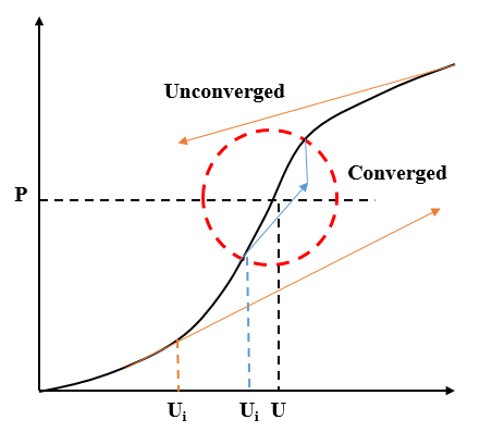
Figure: Convergence Radius

Following strategies are beneficial to carry out converge solution:

Apply load incrementally as discussed (refer determine 2, case 2) Use convergence enhancement equipment to growth radius of convergence.

Nonlinear touch settings along with interface treatment, stabilization damping factors, etc.

You can acquire convergence with above techniques however you want to constantly ensure that it'll now no longer have an effect on the accuracy of the solution.

Essential steps in nonlinear analysis:

I admit that I generally begin with nonlinear geometry due to the fact that is how I were given into this. But I additionally understand that its miles a whole lot greater possibly which you are after nonlinear fabric, so let’s provide it a swing! There are a whole lot of extraordinary nonlinear fabric models. I can’t even listing them all, now no longer to say understanding them in-depth.

This is a part of FEA-magic BTW. You can effortlessly be a professional in a selected area of interest of FEA, and that is so cool! What I’m certain approximately but is, that at the “simple level” of nonlinearity this all is going approximately the stress-pressure relationship.

Each fabric has a stress-pressure curve, generally received from tensile checks in labs. I will admit that it’s now no longer clean to locate exact FREE studies on-line on many materials.

If you're studying you can “guess” an approximate curve and flow on. Just recall now no longer to base your real layout on facts which you guessed! But the above hassle is additionally, why I like metal so a whole lot. It’s a completely properly researched fabric, and stress-pressure curves are widely known and documented. This makes it an ideal fabric to begin with.

Load-displacement relation

The stiffness of the analyzed shape isn't steady and varies with the carried out masses. The displacements are large (translations and rotations) and aren't associated with the unique stiffness of the shape.

Stress-strain relation

Stresses and traces aren't associated with a linear function.

Scalability

The consequences of a nonlinear evaluation cannot be scaled.

Superposition

The precept of superposition cannot be carried out. If a load P1 produces a displacement d1 and a load P2 a displacement d2, then the burden P1 + P2 will now no longer motive a displacement d1 + d2.

Initial state of stress

The preliminary kingdom of stress (residual stresses, temperature, pre-stressing) can be extraordinarily critical with inside the universal reaction.

Load history

The shape’s reaction is associated with the burden history: its miles stimulated through the loading collection. When numerous subcases are carried out in collection with inside the shape, the cease of a subcase is the preliminary circumstance for the following subcase.

Reversibility

The deformation of the shape isn't completely reversible as soon as the carried out masses are removed.

Solution settings

The outside masses are carried out in small increments, and iterations are done to make certain that equilibrium is happy at every load increment. Solution tracking through the person is needed to make certain convergence.

The computing time is generally large. While linear troubles usually have a completely unique answer, a nonlinear hassle may now no longer. In fact, the iterative and incremental approaches used to resolve nonlinear troubles won't converge and might even produce a wrong answer at convergence.

Key Takeaways:

• Additionally, they may be insensitive to huge inflexible frame rotations and translations making them very appropriate for simulations wherein there's additionally geometric nonlinearity.
• Using the Newton method, it frequently takes Abacus/Standard numerous iterations to decide an appropriate method to whenever increment.
• At the quilt of every increment the shape is in (approximate) equilibrium and outcomes are to be had for writing to the restart, data, outcomes, or output database files.
• In case of nonlinear simulation, the stiffness of the shape isn't regular with recognize to loading (pressure as opposed to displacement plot isn't as immediately line).
• The deformation of the shape isn't completely reversible as soon as the carried out masses are removed.

5.3 Dynamic analysis: Introduction to dynamic analysis, Comparison of static and dynamic analysis

The time period dynamic FEA pertains to a number effective simulation strategies that may be carried out to even complicated engineering systems. Dynamic evaluation is used to assess the effect of temporary masses or to layout out capacity noise and vibration problems.

As skilled improvement engineers our contribution to a dynamic assessment not often stops on the evaluation output. We robotically paintings along customers to discover layout answers which can be practical and provide authentic business benefits: Vibration evaluation checking out is high priced.

Carry out dynamics evaluation at layout level can keep away from or lessen of the requirement and the price for rig checking out.

To examine the shape at layout level can keep away from high priced errors in actual use of the product. Modal evaluation is used to discover herbal frequencies.

This is an effective device which lets in engineer to layout the product for the motive warding off excitation to be coincide with the herbal frequencies of the shape consequently remove or minimize immoderate vibration. Animations may be without problems produced to offer precious perception into how the shape will behave while excited. Harmonic reaction evaluation is used to decide the steady-country reaction of a linear shape to sinusoidal masses, and allows the assessment of resistance to sustained compelled vibration.

Rotor dynamic evaluation is critical while designing or troubleshooting rotating systems. By modelling the rotating geometry and its dynamic characteristics, which include stiffness and damping, the important speeds may be predicted. Design changes may be made to keep away from the rotor non-stop strolling at the ones important speeds.

The FSI (Fluid Structure Interface) characteristic in ANSYS lets in the dynamics fluid loading situation to be transferred to the shape as dynamic loading conditions, which make a few complicated research regarding fluid / shape interplay to be carried out. Trivia offer FEA consulting offerings and has a whole lot of revel in in dynamic evaluation. If you would really like to realize greater please experience unfastened to name or email (touch info below). Our skilled engineers can be satisfied to assist you. Alternatively, you can favor to use our easy enquiry form.

Equations of Motion

The primary styles of movement in a dynamic gadget are displacement u and the primary and 2nd derivatives of displacement with recognize to time.

These derivatives are pace and acceleration, respectively, given below: First and 2nd derivatives of displacement with recognize to time (1-1) Velocity and Acceleration

Velocity also can be defined because the slope of the displacement curve. Similarly, acceleration is the charge of alternate of the rate with recognize to time, or the slope of the rate curve.

Single Degree-of-Freedom System

The maximum easy illustration of a dynamic gadget is a unmarried degree-of-freedom (SDOF) gadget. In an SDOF gadget, the time-various displacement of the shape is described with the aid of using one thing of movement u(t). Velocity u̇(t) and acceleration ü(t) are derived from the displacement.

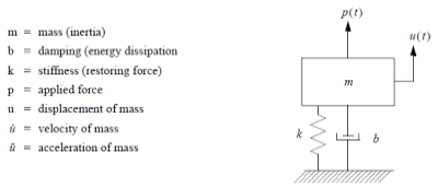
Figure. Singe Degree-of-Freedom (SDOF) System

Dynamic and Static Degrees-of-Freedom

Mass and damping are related to the movement of a dynamic machine. Degrees-of-freedom with mass or damping are regularly known as dynamic degrees-of-freedom; degrees-of-freedom with stiffness are known as static degrees-of-freedom.

It is possible (and regularly desirable) in fashions of complicated structures to have fewer dynamic degrees-of-freedom than static degrees-of-freedom. The 4 fundamental additives of a dynamic machine are mass, power dissipation (damper), resistance (spring), and implemented load. The equilibrium equation representing the dynamic movement of the machine is referred to as the equation of movement.

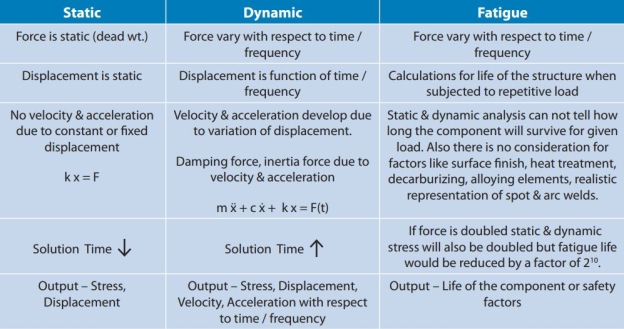
Comparison of static and dynamic analysis:

When accomplishing FEA, the choice ought to be made as to whether or not a static evaluation or a dynamic evaluation is required. There are numerous key variations among the two.

A static evaluation can best be accomplished if the gadget being simulated does now no longer rely on time, and if the hundreds being carried out are constant. In a dynamic evaluation, the gadget itself, the burden application, or each may alternate with time. In a dynamic evaluation, the inertial hundreds advanced with the aid of using the gadget because of acceleration are taken into account.

Mathematically, the distinction among static and dynamic evaluation is that during a static evaluation, best the stiffness matrix of the FEA version is solved.

In a dynamic evaluation, similarly to the stiffness matrix, the mass matrix (and damping matrix, if now no longer zero) is solved as well. That is one of the motives why dynamic analyses require greater computational time than static analyses, for the identical structure.

• Well, I desire you understand the primary distinction of physics among the phrases Static and dynamic. (Static frame is a frame that's at relaxation and dynamic frame is a frame that's in movement.) In FEM or FEA the very last output we preference is the sturdiness of the frame. We version the additives of a frame thinking about all its connections and features.
• The FEA version have to be approximate to the actual version in phrases of weight, rigidity, elasticity etc. So, to test the sturdiness of the version previous to its production we can cross for evaluation for the version.
• Analysis is not anything however the verification of responses for specific load situations that frame may fit via with inside the actual lifestyles applications.
• We anticipate the weight situations and observe the identical load at the version in FEA and sooner or later we test for its fatigue disasters via way of means of soliciting for outputs like displacement, stress, plastic pressure, lifestyles cycles etc.
• So, the loading situations are implemented in solid situation of the frame in addition to in dynamic situations of the frame. Static evaluation is accomplished assuming that the frame is at relaxation i.e. load implemented is a static one and the principle goal of this evaluation is its fatigue failure.
• Dynamic evaluation is accomplished assuming the frame is in movement i.e. dynamic loading is assumed.
• Types of evaluation carried out in the course of static situation are Static 1g loading, 5g loading, static aspect evaluation, regular nation warmth switch evaluation etc.
• Types of evaluation carried out in the course of dynamic situations of the frame are Frequency reaction evaluation,
• Thermo mechanical failure evaluation etc.,
• After appearing static evaluation, we examine the outputs like most displacement below that loading situation, stresses evolved because of that deformation, response forces on the solving vicinity of the frame etc.

Key Takeaways:

• The FSI (Fluid Structure Interface) characteristic in ANSYS lets in the dynamics fluid loading situation to be transferred to the shape as dynamic loading conditions, which make a few complicated research regarding fluid / shape interplay to be carried out. Trivia offer FEA
• These derivatives are pace and acceleration, respectively, given below: First and 2nd derivatives of displacement with recognize to time (1-1) Velocity and Acceleration
• The equilibrium equation representing the dynamic movement of the machine is referred to as the equation of movement.

• Dynamic evaluation is accomplished assuming the frame is in movement i.e. dynamic loading is assumed.

5.4 Time domain and frequency domain, types of loading, simple harmonic motion, free vibration, Boundary conditions of free vibration, solution:

Time Domain:

Time area refers back to the evaluation of mathematical functions, bodily alerts or time collection of financial or environmental data, with admire to time. In the time area, the sign or function's fee is understood for all actual numbers, for the case of non-stop time, or at diverse separate instants with inside the case of discrete time.

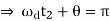
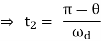
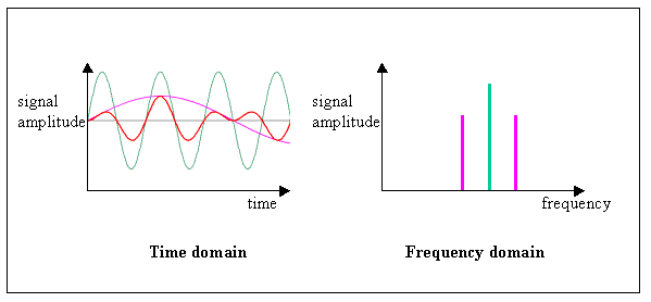
A time-area graph indicates how a sign adjustments with time, while a frequency-area graph indicates how a great deal of the sign lies inside every given frequency band over a number frequencies.

In this chapter, let us discuss the time domain specifications of the second order system. The step response of the second order system for the underdamped case is shown in the following figure.

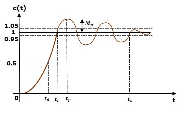
All the time area specs are represented on this figure. The reaction as much as the settling time is called brief reaction and the reaction after the settling time is called constant country reaction.

Delay Time

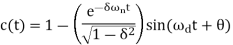
It is the time required for the reaction to attain 1/2 of of its very last price from the 0 instant. It is denoted with the aid of using td. Consider the step reaction of the second one order device for t ≥ 0, when ‘δ’ lies among 0 and one.

c(t) = 1-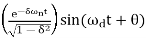

The final value of the step response is one.

Therefore, at t = td , the value of the step response will be 0.5. Substitute, these values in the above equation.

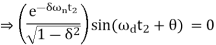
c(td) = 0.5 = 1-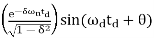

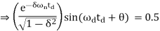
By using linear approximation, you will get the delay time td  as

Rise Time

It is the time required for the reaction to upward thrust from 0% to 100% of its very last price. This is relevant for the under-damped systems.

For the over-damped systems, don't forget the length from 10% to 90% of the very last price. Rise time is denoted with the aid of using tr.

At t = t1 = 0, c(t) = 0. We realize that the very last price of the step reaction is one. Therefore, at t=t2, the price of step reaction is one.

c(t2) = 1 = 1-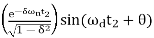

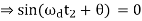
Substitute t1 and t2 values in the following equation of  rise time.

tr = t2 – t1

∴tr=π−θ/ωd

Frequency Domain:

In physics, electronics, manage structures engineering, and statistics, the frequency area refers back to the evaluation of mathematical capabilities or indicators with recognize to frequency, in preference to time.

Put simply, a time-area graph indicates how a sign modifications over time, while a frequency-area graph indicates how an awful lot of the sign lies inside every given frequency band over quite a number frequencies.

A frequency-area illustration also can encompass data at the segment shift that ought to be carried out to every sinusoid so as to be capable of recombine the frequency additives to get better the authentic time sign. A given feature or sign may be transformed among the time and frequency domain names with a couple of mathematical operators known as transforms.

An instance is the Fourier rework, which converts a time feature right into a sum or imperative of sine waves of various frequencies, every of which represents a frequency component. The "spectrum" of frequency additives is the frequency-area illustration of the sign.

The inverse Fourier rework converts the frequency-area feature again to the time-area feature. A spectrum analyzer is a device usually used to visualize digital indicators with inside the frequency area. Some specialized sign processing strategies use transforms that bring about a joint time–frequency area, with the instant frequency being a key hyperlink among the time area and the frequency area.

The Frequency location works with the useful resource of the use of allowing a example of the qualitative behavior of a tool, similarly to trends of the way the tool response to adjustments in bandwidth, gain, section shift, harmonics, etc. A location in which the frequency location is used for graphical example is in music.

Often audio producers and engineers display an audio signal interior a frequency location a very good manner to better understand the shape and character of an audio signal.

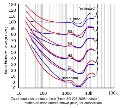
For example, auditory sounds exist among more than a few 20-20,000Hz, and a few frequencies are tougher for the human ear to withstand. The frequency 3,400Hz is a harsh frequency (the sound of toddlers crying), and the human ear is in particular tuned to reply viscerally to that sound. An audio engineer may also lessen the electricity of that frequency with inside the frequency area the usage of an audio equalizer. By showing the audio sign with inside the frequency area, an engineer can raise and decrease indicators to make the sounds extra first-class for the human ear. The Fletcher-Munson curve is a extensively used characteristic that lays atop the frequency area that audio engineers regularly reference whilst blending diverse frequencies.

Types of loading:

Nodal Loads

For structural evaluation a nodal load may be a nodal pressure or a nodal moment. These masses may be described in each node with inside the version wherein a respective foundation is described (translations for pressure and rotations for moments).

Weight Loads

The extent of the factors is calculated via way of means of Diana. A weight load can be described in numerous load instances, however the path and acceleration are continually equal. When specific acceleration masses are carried out in specific guidelines and/or with specific acceleration values, equal acceleration masses may be exact as alternative.

Direction of gravity and gravity acceleration are used to transform stress heads into pore-pressures for groundwater-float evaluation and consequently should be particular with inside the version.

Equivalent Acceleration Loads

An equal acceleration load specification calls for the definition of the path of gravity, gravity acceleration and mass density for factors. An equal acceleration load can be described in numerous load instances, with specific accelerations and guidelines of acceleration.

Even specific equal acceleration masses can be described with inside the equal load case. This in opposite to weight masses for which the gravity acceleration and gravity path should be the equal for all weight masses with inside the version.

Centrifugal Loads

A centrifugal load specification calls for the definition of axis of centrifugation, the rotation velocity and mass density for factors. A centrifugal load can be described in numerous load instances, with specific accelerations and guidelines of acceleration. Only one centrifugal load can be laid out in a load case.

Fixed Displacement or Deformation Loads

These levels of freedom should be recognized as constraint levels of freedom, with the intention to make certain that the constant displacement diploma of freedom is taken into consideration as a constraint nodal variable [Eq. (7.1)].

That manner that for a linear elastic evaluation with numerous load instances, for which in best one load case a deformation load is described, the levels of freedom for which a deformation load is described may be constraint for all load instances.

This technique has the benefit that evaluation time is stored due to the fact the set of constraint and unconstraint variable is equal for all load instances or proper hand aspect vectors. As an outcome the matrix want to be decomposed best one time, while for each load case best the substitution will to be done.

Prescribed Acceleration

Prescribed accelerations may be utilized in temporary dynamic evaluation to version non-uniform nodal accelerations. A spatial feature may be connected to this property [§ 5.6]. Prescribed accelerations should be exact as supports. Consequently they may have a 0 displacement for all instances, except acceleration values are exact. Prescribed accelerations cannot be blended with base acceleration masses and stuck displacement or deformation masses with inside the equal load set.

Distributed masses

Loads may be disbursed in traces and surfaces. Force line masses are immediately carried out with the real values of the weight with inside the detail nodes. A spatial feature [§ 5.6] may be connected to those masses.

Mobile Loads

In bridge design, cellular (or moving) masses are regularly carried out to get the intense values of evaluation outcomes like strains, stresses, or guide reactions. The utility of cellular masses is difficulty to the subsequent restrictions.

Mobile masses can best act on beam factors. It is authorized to attach different factors to the beam factors on which a cellular load acts, as an instance in a plate version of a bridge.

When the stiffness of the beam factors is negligible in evaluation to the plate factors, the best feature of the beam factors is to outline the cellular load pathway. Mobile masses can best be carried out in everyday linear static evaluation. Only one cellular load consistent with load case can be described. If a load case incorporates a cellular load, no different masses are allowed on this load case.

Simple harmonic motion, free vibration, Boundary conditions of free vibration, solution

Simple Harmonic Motion or SHM is described as a movement wherein the restoring pressure is immediately proportional to the displacement of the frame from its suggest role. The route of this restoring pressure is continually toward the suggest role. The acceleration of a particle executing easy harmonic movement is given with the aid of using,

a(t) = -ω2 x(t).

It is a unique case of oscillatory movement. All the Simple Harmonic Motions are oscillatory and additionally periodic however now no longer all oscillatory motions are SHM. Oscillatory movement is likewise known as the harmonic movement of all of the oscillatory motions in which the maximum crucial one is easy harmonic movement (SHM).

In this form of oscillatory movement displacement, pace and acceleration and pressure vary (w.r.t time) in a manner that may be defined with the aid of using both sine (and) the cosine capabilities together known as sinusoids.

Behavior of composites to excessive speed effect continues to be now no longer properly understood. Very few literatures are mentioned on this connection. Starting from manufacturing, and at some stage in their layout life, those systems are at risk of notably temporary loading which includes device drop and different sorts of effect.

Such conditions fall below wave propagation troubles and traits that differentiates this hassle from traditional dynamic reaction troubles are excessive frequency content material of loading records and the section transformation for the duration of propagation. The dynamics of deep beam systems subjected to excessive frequency loading (or effect) introduces sure consequences that are absent of their essential counterparts.

High frequency contents require huge device length in FE formula to seize all of the better modes. Hence the detail length must be akin to wavelengths that are very small at excessive frequencies.

Such troubles are historically solved in frequency area and one such approach is the spectral detail approach (SEM) (see [25] for isotropic Timoshenko beam and for composite Euler–Bernoulli beam). Using SEM, it's miles less complicated to seize crucial traits of beam temporary dynamics.

However, spectral detail formulations, that are primarily based totally on specific answers to the governing wave equations with inside the converted frequency area is to be had until date simplest for few structural elements (which includes rods, beams, cylinders, etc.).

The paper is prepared as follows. First, the finite detail formula is outlined. Here, we derive the precise form capabilities bobbing up from specific answers to the governing equations. Using those form capabilities, the precise stiffness matrix and regular mass matrix and cargo matrix are received. Next, static, unfastened vibration and wave propagation troubles are solved the usage of this detail. Results of static and unfastened vibration troubles are in comparison with the ones to be had in current literatures

Wave propagation answers are in comparison with 2D aircraft strain FE answers. Next, composite beams with structural discontinuities which includes ply-drops, inflexible and lap joints are analyzed. A global/nearby approach is used to version delamination. Natural frequencies of a delaminated beam received the usage of this technique is in comparison with the end result mentioned with inside the literature.

Mode I and Mode II strain depth elements are computed from J-crucial on the global/nearby interface. Important conclusions are made together with dialogue on similarly scope of research to apply such technique for quicker and cost-powerful FE analysis.

Free vibration, which gives an exceptional opportunity of harnessing inexperienced electricity, has been receiving great interest for the beyond few decades.

Although efficient, sun and wind electricity have their personal regulations while wished everywhere and every time which includes interior or at night. Moreover, they're the sources of large-scale energy plants (>one hundred MW) that simply fulfill the electricity requirement of small-scale transportable gadgets.

On the opposite hand, unfastened vibration is constantly determined in any surroundings. Utilizing unfastened vibration, harnessing electricity might be an exceptional capacity for self-powered digital gadgets which have a plethora of applications, which includes sensors, detectors, structural fitness monitoring, scientific implants, etc.

Therefore, piezoelectric electricity harvester which matches beneath unfastened vibration is one of the predominant regions of electricity source, which has been in large part exploited for the beyond few years.

Furthermore, it stays the maximum extensively researched harvesting generation due to its high-voltage output, high-energy density, ease in operation, and evolved thin- and thick-movie deposition methods.

Apart from piezoelectricity, the opposite manner to generate energy from vibration is electromagnetic induction whose transduction precept is primarily based totally at the famous Faraday's law.

Scavenging electricity through this approach may be found out through coupling an everlasting magnet and a solenoid in movement relative to every other. Although this approach has numerous blessings in phrases of low frequencies (2–20 Hz) and small impedance, it suffers from the problems in integration with microelectromechanical (MEMS) technologies.

Hence, few options of harnessing electricity have additionally been explored which gives massive promise with inside the coming generations for MEMS utility and microelectronic gadgets.

Among them, electricity harvesting the use of microfluidic droplet is vital to mention. Lately, an exceptional deal of studies paintings has been committed to scavenge electricity through rolling and actuating droplet on diverse surfaces through exploiting diverse interfacial phenomena which includes hydrophobic–hydrophilic interface, touch electrification, electro kinetic capacity, etc.

Therefore, its miles of maximum significance to summarize the literature specializing in the subject above. Before discussing the information of droplet primarily based totally electricity harvesting, it's miles vital to speak about the fundamental transduction precept, kinds of substances used, idea of hydrophobicity and hydrophobicity, electro wetting, bulge instability, etc. In the subsequent section, we can in brief speak the above subject matter earlier than coming to the case research of electricity harvesting through droplets.

Boundary Conditions:

Clamped boundary

The boundary conditions are formulated as follows:

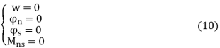
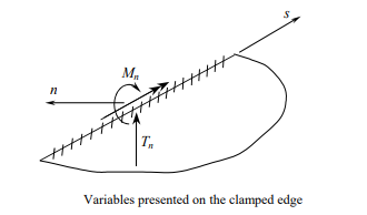
The unknown variables are: the bending moment M­n and the shear force Tn.

Simply-supported boundary

The boundary conditions are formulated as follows:

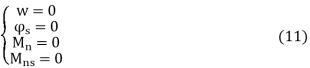
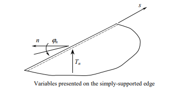
The unknown variables are: the shear force Tn and the angle of rotation in direction n,

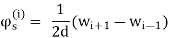
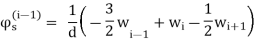
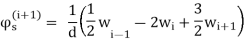
Free boundary

The boundary conditions are formulated as follows:

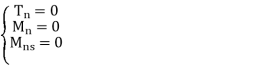
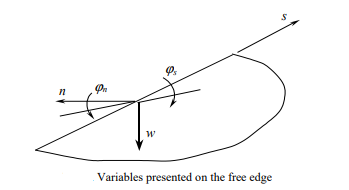
The unknown variables are: the deflection w and the angles of rotation ϕn, ϕs. Because the relation between ϕs and w is known, ϕs= ∂w/∂s, there are only two independent values: w and ϕn. After discretization of a plate boundary into constant elements having the same length, parameter (y)              ∂w/∂s can be calculated approximately by constructing a differential expression using deflections of three neighboring nodes.

Key Takeaways:

• A time-area graph indicates how a sign adjustments with time, while a frequency-area graph indicates how a great deal of the sign lies inside every given frequency band over a number frequencies.
• It is the time required for the reaction to attain 1/2 of of its very last price from the 0 instant. It is denoted with the aid of using td.
• It is the time required for the reaction to upward thrust from 0% to 100% of its very last price. This is relevant for the under-damped systems.
• An instance is the Fourier rework, which converts a time feature right into a sum or imperative of sine waves of various frequencies, every of which represents a frequency component. The "spectrum" of frequency additives is the frequency-area illustration of the sign.
• This in opposite to weight masses for which the gravity acceleration and gravity path should be the equal for all weight masses with inside the version.
• That manner that for a linear elastic evaluation with numerous load instances, for which in best one load case a deformation load is described, the levels of freedom for which a deformation load is described may be constraint for all load instances.

References:

1. K. J. Bathe, Finite Element Procedure, Prentice-Hall of India (P) Ltd., New Delhi, 1996.

2. Cook R. D., Finite Element Modeling for Stress Analysis, John Wiley and Sons Inc, 1995.

3. G.R. Liu S. S. Quek, The Finite Element Method- A Practical Course, Butterworth Heinemann, 2013.

4. Fagan M. J., Finite Element Analysis Theory and Practice, Harlow Pearson/Prentice Hall, 2012.

5. S. Moaveni, Finite element analysis, theory and application with Ansys, Pearson, Third Edition, 2011.

6. David V. Hutton, Fundamental of Finite Element Analysis, Tata McGraw-Hill, 2017.