Unit - 4
Time and Frequency Domain Analysis
For a second order control system, the total time response is analysed by its transient as well as ready state response.
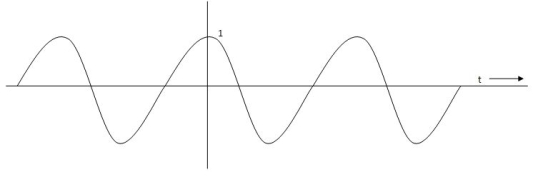
Any system which contains energy along elements (L1 c etc) if suffer any disturbance in the energy state effect at the input end as at this output or at both the ends takes source time to change in thus form one state other. This change its then is called as Transient times and the values of reverent and voltage during this period is Transient Response.
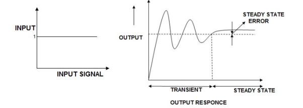
Fig:1 Transient Response
The above fig: A clearly shows steady state response is that part of response when the transient has died. If the steady star response of the output does not match with input, then the system has steady state errors.
Consider the following open loop system –
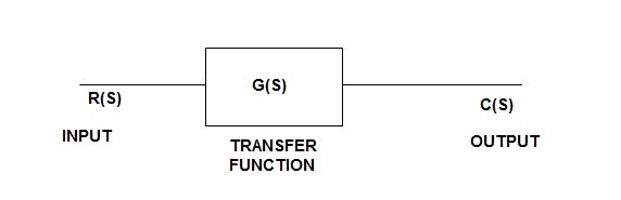
Fig 2 Open loop system block diagram
L-1[c(s)] = L-1[ G(s) R (S)]
C(t) = L-1[ G(S) Q (s)]
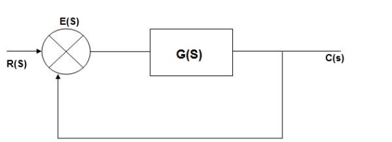
Fig 3 Closed loop system block diagram
E(s) = R(s) –c(s) [ error signal]
C(S)= [ R(s)- c(Q)] G(s)
C(s) = R(s) G(s)- c(s) G(s)
C(s) [ 1+G(s)] = R(s) G(s)
C(s)/R(s) = G(s)/1+G(s)
C(s)/R(s) = G(s)/1+G(s)
E(s) = R(s)- c(s)
=R(s)-R(s) G(s)/1+G (s0
E(s) = R(s) [1/1+G(s)
If no error then E(s) = 0, f(t) = 0 Hence, r(t) = c(t)
Key takeaway
The error signal is the difference between the unity feedback signal and input signal.
Standard Test Inputs of Time Domain Analysis
The Impulse signal, Ramp signal, unit step and parabolic signals are used as the standard test signals. All these signals are explained below.
Impulse Signal:
This signal has zero amplitude everywhere except at the origin. Fig below shown the representation of Impulse signal.
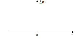
Fig 4 Unit Impulse Signal
The mathematical representations
A (t) = 0 for t ≠0
 dt = A e
Where A represent energy or area of the Laplace Transform of Impulse signal is
L [A (t)] = A
Unit Impulse Signal:
If A = 1
 (t) = 0 for t ≠0
L [ (t)] = 1
The transfer function of a linear time invariant
System is the Laplace transform of the impulse response of the system. If a unit impulse signal is applied to system, then Laplace transform of the output c(s) is the transfer function G(s)
As we know G(s) = c(s)/R(S)
r(t) =  (t)
(t)
R(s) = L [ (t)] = 1
:. G(S) = C(s)
(b) Step signal:
Step signal of size A is a signal that change from zero level to A in zero time and stays there forever.
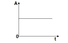
Fig 5 Unit Step Signal
r(t)= A t >=0
=0 t<0
L[r(t)] = R(s) = A/s
Unit Step Signal: If the magnitude of the slip signal is I then it is called unit step signal.
u(t) = 1
t>=0
t<0
L[u(t)] = 1/s
(c) Ramp Signal:
The vamp signal increase linearly with time from initial value of zero at t= 0 as shown in fig is below
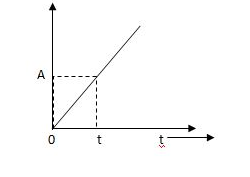
Fig 6 Ramp Signal
r(t) = At t>=0
=0 t<0
A is the slope of the line The Laplace transform of ramp signal is
L[r(t)] = R(s) = A/s2
(d) Parabolic Signal:
The instantaneous value of a parabolic signal varies as square of the time from an initial value of zero t=0. The signal representation in fig 14 below.
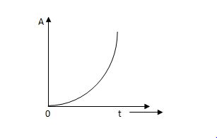
Fig 7 Parabolic Signal
r(t) At2 t>=0
=0 t<0
Then Laplace Transform is given as
R(s) = L[At2] = 2A/s3
If no error then E(t) =0, R(t) = c(t), output is tracking the input.
Steady state Errors signal (ess): - (t  )
)
Ess = t  e(t)
e(t)
Using final values, the theorem
 = ess =
  S.E (s)
ess=  S[R(s)/1+G/(s)]
Key takeaway
If no error then E(t) =0, R(t) = c(t), output is tracking the input.
Steady state Errors signal (ess): - (t  )
)
Ess = t  e(t)
e(t)
Using final values, the theorem
 = ess =
  S.E (s)
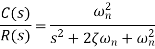
Unit step Response analysis via Transient response specifications
OLTF G(s) = k/s(1+TS)
CLTFC(s)/R(s) = k/k+s(1+Ts)
= k/s2+ s/T +k/T
Comparing above equation with standard 2nd order eqn
CLTF = wn2/s2+2rs wns+wn2
Standard 2nd order equation
CEs2+2 wn s+wn2= 0
S= -2 wn±
wn± /2
/2
=2 wn±2wn
 /2
/2
S= wn±wn
wn±wn
S= - wn±wn
wn±wn
S= - wn ±wn
S= - wn ±gwn
Standard eqn:
T(s) = wn2/s2+2 wns+wn2
Our eqn T(s) = K/T/s2+1/T s+ K/T
Wn2 = k/T
2 wn = 1/T
2 k/T = 1/T
 k/T = 1/2T
 = 1/2T
  T/K
T/K
 = 1
= 1 2KT
2KT
Graphically showing the position of loops s1, s2 for offered of
As the characteristic Eqn (location of poles) is dependent only on (wn constant for a given system)
S1 = - wn + jwn
  1-
1- 2
2
S2= - wn - jwn
 1-
1- 2
2
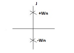
CASE 1: ( =0)
=0)
S1=jwn, S2, = -jwn
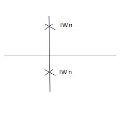
Fig 8 Location of poles for  =0
=0
Undamped
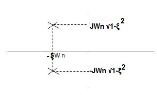
CASE 2:(0< <1)
<1)
S1= -wn + jwn  0.75
0.75
=-wn/2 +jwn (0.26)
S2 = -wn/2 – jwn (0.86)
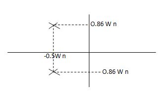
Fig 9 Location of poles for  <1
<1
CASE:3 ( =1)
=1)
S1= S2 = - wn = -wn
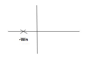
Fig 10 Location of poles for  =1
=1
CASE4: ( =-2)
=-2)
S1 = -2wn +jwn  -3
-3
=-2wn – jwn (1.73)
S1 = -3.73wn
S2 = -2wn –jwn  -3
-3
= -2wn + jwn (1.73)
= -0.27  wn
wn
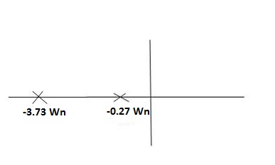
Fig 11 Location of poles for  >1
>1
Overdamped
All practical systems are 2 order to, if R(e) =  (t) R(s) = 1: CLTF = 2nd order st eqn and hence already the system is possible.
CLTF = e(s)/ R(s) = wn2/s2+2 wns+wn2
Now calculating c(s), c(t) for different values of input
1) Impulse I/p
R(t) =  (t)
(t)
R(s) = 1
C(s) = R(s) wn2/s2+2 wns+wn2
C(s) = wn2/s2 +2 wn+wn2
Under this i/p (R(t) =  (t)) the output varies with different values of
  . So,
. So,
CONDITION 1: ( =0)
=0)
C(s) =wn2/s2 +wn2
Os2 +wn2 =0
S=+-jwn
C(t) = wn sinwnt
Sinwnt
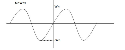
Fig 12 Undamped oscillations
As there in no damping i.e., oscillations at t= 0 are some at t  so, called UNDAMPED
CONDITION 2: 0<<1
c(s) = R(s) wn2/s22 wn+wn2 R(t) =
  (t)
(t)
R(s) =1
C(s) = wn2/s2+2 wns+wn2
CE
S2+2 wns +wn2 =0
S2, S1 = - wn ±jwn
  1-
1- 2
2
C(t) = e- wnt sin (wn
  )t
)t
Wd=wn )
)
C(t)=e- wnt sin (wdt)
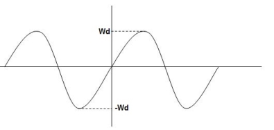
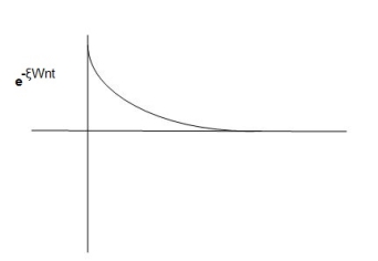
Fig 13 Underdamped oscillations
The oscillations are present but at t- infinity the Oscillations are 0 so, it is UNDERDAMPED
CONDITION 3:  =1
=1
C(s) = R(s) wn2/s2+2 wns+wn2
C(s)=wn2/S2 +2wns+wn2
=wn2/ (s +wn)2
CE S= -Wn
Diagram
C(t)= w2n / (
 )2
)2
C(t)=
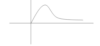
Fig 14 Critically damped oscillations
No damping obtained at  so is called CRITICALLY DAMPED.
CONDITIONS 4: >1
>1
C(s) = wn2/s22 wnS+Wn2
S1, s2 =  WN+-jwn
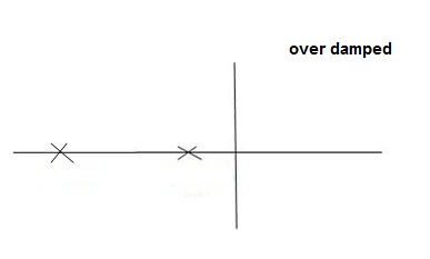
Fig 15 location of poles for over damped oscillations
a) UNIT Step Input:
R(s) = 1/s
C(s)/R(s) = wn2/s2+2 wns+wn2
C(s) = R(s) wn2 /s2 +2 wns+wn2
C(s) = R(s) wn2/s2+2 wns+wn2
C(s) = R(s) wn2/s2+2 wns+wn2
C(s) = wn2s(s2+2 wns+wn2)
C(t) = 1- e wnt/
wnt/ 1-es2 sin (wdt + ø)
Wd = wn 1-
1- 2
2
Ø= 
Where
Wd = Damping frequency of oscillations
Wn = natural frequency of oscillations
 wn = damping coefficient.
T= Time constant
Condition 1 = 0
= 0
C(s) = wn2 /s(s2+wn2)
C(t) = 1- e° sin wdt +ø
C(t)= 1- sin (wn +90)
C(t) = 1+cos wnt
Constant
C(t) = 1+constant
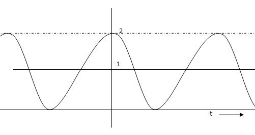
Fig 16 C(t) = 1+cos wnt
Condition 2: 0< <1
<1
C(s) =  /s2+
/s2+ wns +wn2
C(s) =1/s – s+ wn/s2+
 wns +wn2
=1/s – s+ wn/(s+
 wn)2+wd2-
  wn/(s+
 wn2) +wd2
Wd = wn  1-
1- 2
2
Taking Laplace inverse of above equation
L --1 s+ wn/(s+
 wn) +wd2= e-
 wnt cos wdt
L-1 s+ wn/(s+
 wn)2+wd2 = e-
 wnt sinWdt
C(t) = 1-e- wnt [coswdt +
 /
/ 1-
1- 2 sinwdt]
= 1-e wnt /
wnt / 1-
1- 2 sin [wdt +
  1-
1- 2/
2/ ] t>=0
C(t) = 1-e wnt/
wnt/ 1-
1- 2 sin(wdt+ø)
Ø =  1+
1+ 2/
2/
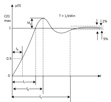
Fig 17. Transient Response of second order system
Specifications:
1) Rise Time (tp): The time taken by the output to reach the already status value for the first time is known as Rise time.
C(t) = 1-e- wnt/
wnt/ 1-
1- 2 sin (wdt+ø)
Sin (wd +ø) = 0
Wdt +ø = n
tr =n -ø/wd
-ø/wd
For first time so, n=1.
tr =  -ø/wd
-ø/wd
T=1/
2) Peak Time (tp)
The peak value attained by the output is called peak time. The time required by the output to reach this value is lp.
d(cct) /dt = 0 (maxima)
d(t)/dt = peak value
tp = n /wd for n=1
tp =  wd
wd
3) Peak Overshoot Value:
Maximum deviation of output from steady state value is called peak overshoot value (Mp).
(ltp) = 1 = Mp
(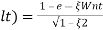 Sin (Wat + φ)
(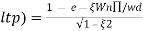 Sin (Wd∏/Wd + φ)
Mp = e-∏ξ / √1 –ξ2
Condition 3 ξ = 1
C (S) = R (S) Wn2 / S2 + 2ξWnS + Wn2
C (S) = Wn2 / S (S2 + 2WnS + Wn2) [ R(S) = 1/S]
C (S) = Wn2 / S (S2 + Wn2)
C (t) = 1 – e-Wnt + tWne-Wnt
The response is critically damped.
4) Settling Time (ts):
ts = 3 / ξWn (5%)
ts = 4 / ξWn (2%)
Key takeaway
Rise Time tr =  -ø/wd
-ø/wd
Peak Time tp = n /wd for n=1
tp =  wd
wd
Peak Overshoot Value
Mp% = e-∏ξ / √1 –ξ2
Settling Time
ts = 3 / ξWn (5%)
ts = 4 / ξWn (2%)
Examples
Q.1. The open loop transfer function of a system with unity feedback gain G (S) = 20 / S2 + 5S + 4. Determine the ξ, Mp, tr, tp.
Sol: Finding closed loop transfer function,
C (S) / R (S) = G (S) / 1 + G (S) + H (S)
As it is unity feedback so, H(S) = 1
C(S)/R(S) = G(S)/1 + G(S)
= 20/S2 + 5S + 4/1 + 20/S2 + 5S + 4
C(S)/R(S) = 20/S2 + 5S + 24
Standard equation for second order system,
S2 + 2ξWnS + Wn2 = 0
We have,
S2 + 5S + 24 = 0
Wn2 = 24
Wn = 4.89 rad/sec
2ξWn = 5
(a). ξ = 5/2 x 4.89 = 0.511
(b). Mp% = e-∏ξ / √1 –ξ2 x 100
= e-∏ x 0.511 / √1 – (0.511)2 x 100
Mp% = 15.4%
(c). tr = ∏ - φ / Wd
φ = tan-1√1 – ξ2 / ξ
φ= tan-1√1 – (0.511)2 / (0.511)
φ = 1.03 rad.
tr = ∏ - 1.03/Wd
Wd = Wn√1 – ξ2
= 4.89 √1 – (0.511)2
Wd = 4.20 rad/sec
tr = ∏ - 1.03/4.20
tr = 502.34 msec
(d). tp = ∏/4.20 = 747.9 msec
Q.2. A second order system has Wn = 5 rad/sec and is ξ = 0.7 subjected to unit step input. Find (i) closed loop transfer function. (ii) Peak time (iii) Rise time (iv) Settling time (v) Peak overshoot.
Sol: The closed loop transfer function is
C(S)/R(S) = Wn2 / S2 + 2ξWnS + Wn2
= (5)2 / S2 + 2 x 0.7 x S + (5)2
C(S)/R(S) = 25 / S2 + 7s + 25
(ii). tp = ∏ / Wd
Wd = Wn√1 - ξ2
= 5√1 – (0.7)2
= 3.571 sec
(iii). tr = ∏ - φ/Wd
φ= tan-1√1 – ξ2 / ξ = 0.795 rad
tr = ∏ - 0.795 / 3.571
tr = 0.657 sec
(iv). For 2% settling time
ts = 4 / ξWn = 4 / 0.7 x 5
ts = 1.143 sec
(v). Mp = e-∏ξ / √1 –ξ2 x 100
Mp = 4.59%
Q.3. The open loop transfer function of a unity feedback control system is given by
G(S) = K/S (1 + ST)
Calculate the value by which k should be multiplied so that damping ratio is increased from 0.2 to 0.4?
Sol: C(S)/R(S) = G(S) / 1 + G(S)H(S) H(S) = 1
C(S)/R(S) = K/S (1 + ST) / 1 + K/S (1 + ST)
C(S)/R(S) = K/S (1 + ST) + K
C(S)/R(S) = K/T / S2 + S/T + K/T
For second order system,
S2 + 2ξWnS + Wn2
2ξWn = 1/T
ξ = 1/2WnT
Wn2 = K/T
Wn =√K/T
ξ = 1 / 2√K/T
ξ = 1 / 2 √KT
Forξ1 = 0.2, for ξ2 = 0.4
ξ1 = 1 / 2 √K1T
ξ2 = 1 / 2 √K2T
ξ1/ ξ2 = √K2/K1
K2/K1 = (0.2/0.4)2
K2/K1 = 1 / 4
K1 = 4K2
Q.4. Consider the transfer function C(S)/R(S) = Wn2 / S2 + 2ξWnS + Wn2
Find ξ, Wn so that the system responds to a step input with 5% overshoot and settling time of 4 sec?
Sol:
Mp = 5% = 0.05
Mp = e-∏ξ / √1 –ξ2
0.05 = e-∏ξ / √1 –ξ2
Cn 0.05 = - ∏ξ / √1 –ξ2
-2.99 = - ∏ξ / √1 –ξ2
8.97(1 – ξ2) = ξ2∏2
0.91 – 0.91 ξ2 = ξ2
0.91 = 1.91 ξ2
ξ2 = 0.69
(ii). ts = 4/ ξWn
4 = 4/ ξWn
Wn = 1/ ξ = 1/ 0.69
Wn = 1.45 rad/sec
1>. Resonant Peak (Mr): The maximum value of magnitude is known as Resonant peak. The relative stability of the system can be determined by Mr. The larger the value of Mr the undesirable is the transient response.
2>. Resonant Frequency (Wr): The frequency at which magnitude has maximum value.
3>. Bandwidth: The band of frequencies lying between -3db points.
4>. Cut-off frequency –The frequency at which the magnitude is 3db below its zero frequency.
5>. Cut-off Rate – It is the slope of the log magnitude curve near the cut off frequency.
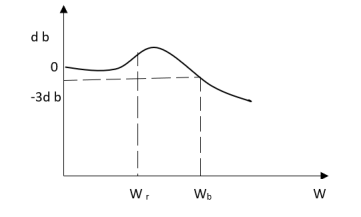
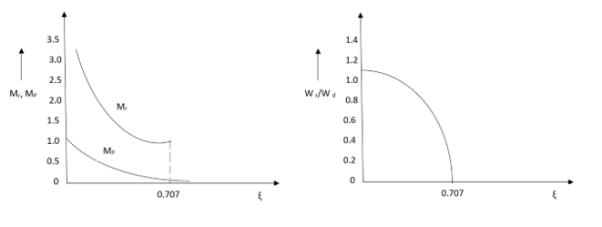
Fig 18 Frequency Domain Specification
Correlation between time domain and frequency domain specifications
The transfer function of second order system is shown as
C(S)/R(S) = W2n / S2 + 2ξWnS + W2n - - (1)
ξ = Ramping factor
Wn = Undamped natural frequency for frequency response let S = jw
C(jw) / R(jw) = W2n / (jw)2 + 2 ξWn(jw) + W2n
Let U = W/Wn above equation becomes
T(jw) = W2n / 1 – U2 + j2 ξU
So,
| T(jw) | = M = 1/√ (1 – u2)2 + (2ξU)2 - - (2)
T(jw) = φ = -tan-1[ 2ξu/(1-u2)] - - (3)
For sinusoidal input the output response for the system is given by
C(t) = 1/√(1-u2)2 + (2ξu)2Sin [wt - tan-1 2ξu/1-u2] - - (4)
The frequency where M has the peak value is known as Resonant frequency Wn. This frequency is given as (from eqn (2)).
DM/du|u=ur = Wr = Wn√(1-2ξ2) - - (5)
From equation (2) the maximum value of magnitude is known as Resonant peak.
Mr = 1/2ξ√1-ξ2 - - (6)
The phase angle at resonant frequency is given as
Φr = - tan-1 [√1-2ξ2/ ξ] - - (7)
As we already know for step response of second order system the value of damped frequency and peak overshoot are given as
Wd = Wn√1-ξ2 - - (8)
Mp = e- πξ2|√1-ξ2 - - (9)
The comparison of Mr and Mp is shown in figure. The two performance indices are correlated as both are functions of the damping factor ξ only. When subjected to step input the system with given value of Mr of its frequency response will exhibit a corresponding value of Mp.
Similarly, the correlation of Wr and Wd is shown in fig (2) for the given input step response [ from eqn (5) & eqn (8)]
Wr/Wd = √ (1- 2ξ2)/(1-ξ2)
Mp = Peak overshoot of step response
Mr = Resonant Peak of frequency response
Wr = Resonant frequency of Frequency response
Wd = Damping frequency of oscillation of step response.
From fig it is clear that for ξ> 1/2, value of Mr does not exist.
Key takeaway
i) Mr and Mp are correlated as both are functions of the damping factor ξ only
Ii) When subjected to step input the system with given value of Mr of its frequency response will exhibit a corresponding value of Mp.
Natural frequency
The natural frequency is defined as the frequency at which a system oscillates when not subjected to a continuous or repeated external force. This frequency can be calculated simply by the following relationship: wn=sqrt(k/m) where k is the stiffness and m is the mass of the system.
Damping frequency
The damped frequency or ringing frequency is the frequency at which a DAMPED system oscillates when not subjected to a continuous or repeated external force. Damped frequency is lower than natural frequency and is calculated using the following relationship: wd=wn*sqrt(1-z) where z is the damping ratio and is defined as the ratio of the system damping to the critical damping coefficient, z=C/Cc where Cc, the critical damping coefficient, is defined as: Cc=2*sqrt(km).
Damping factor
Technically, the damping factor of a system refers to the ratio of nominal loudspeaker impedance to the total impedance driving it (amplifier and speaker cable). In practice, damping is the ability of the amplifier to control speaker motion once signal has stopped. A high damping factor means that the amplifier’s impedance can absorb the electricity generated by speaker coil motion, stopping the speaker’s vibration.
Other points:
- Damping varies with frequency. Some manufacturers publish a damping curve for their amps.
- The effects of damping are most apparent at low frequencies, in the range of the woofer’s resonance. Well damped speakers sound “tighter” in the low end. Low damping factors result in mushy or indistinct bass.
- Speakers connected in series or parallel will experience the same damping factor from the amp. Impedance determines damping factor, not speaker wiring.
- Higher impedance speakers increase system damping factor.
- The damping factors you see published as amp specs are for the amp only, not referenced to an entire system. Higher is better, and you’ll often see quite high numbers, 200, 300, even 3000 or higher.
- System damping factors over 10 are generally acceptable. The higher the better.
Key takeaway
The natural frequency is defined as the frequency at which a system oscillates when not subjected to a continuous or repeated external force.
Second Order Systems
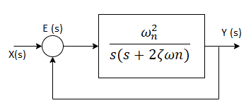
Fig 19 Second order system
The order of a differential equation is the highest degree of derivative present in that equation. A system whose input-output equation is a second order differential equation is called Second Order System.
There are a number of factors that make second order systems important. They are simple and exhibit oscillations and overshoot. Higher order systems are based on second order systems. In case of mechanical second order systems, energy is stored in the form of inertia whereas in case of electrical systems, energy can be stored in a capacitor or inductor.
Standard form of second order system is given by:
Where:
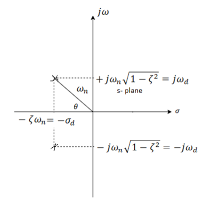

Fig 20 Pole plot for an underdamped second order system
- ωn Is the natural frequency
- Introduction to Second Order Systems 3is the damping ratio
- If 0< Introduction to Second Order Systems 3 <1, system is named as Damped System
- If < Introduction to Second Order Systems 3 =1, system is named as Critically Damped System
- If < Introduction to Second Order Systems 3 >1, system is named as Over Damped System
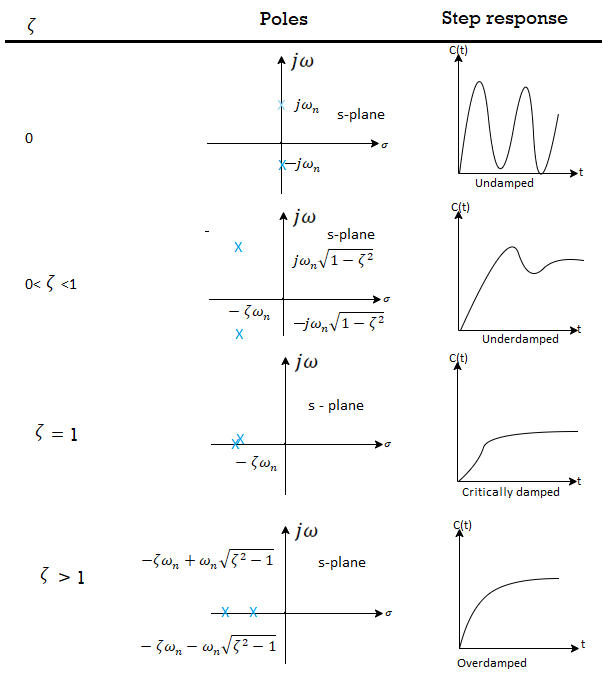
Fig 21 Second order response as a function of damping ratio
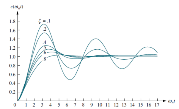
Fig 22 Second order underdamped response for different damping ratio
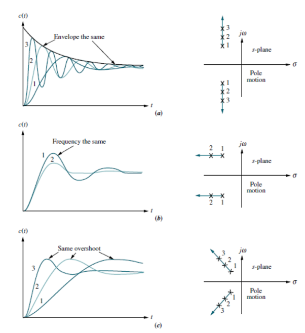
Fig 23 Unit step response of second order system (a) with constant real part (b) imaginary part (c) with constant damping ratio
Let us move the poles to the right or left. Since the imaginary part is now constant, movement of the poles yields the responses of Fig (b). Here the frequency is constant over the range of variation of the real part. As the poles move to the left, the response damps out more rapidly.
Moving the poles along a constant radial line yields the responses shown in Fig(c). Here the percent overshoot remains the same. Notice also that the responses look exactly alike, except for their speed. The farther the poles are from the origin, the more rapid the response.
What is Bode Plot
A Bode plot is a graph commonly used in control system engineering to determine the stability of a control system. A Bode plot maps the frequency response of the system through two graphs – the Bode magnitude plot (expressing the magnitude in decibels) and the Bode phase plot (expressing the phase shift in degrees).
A Bode plot is a standard format for plotting frequency response of LTI systems. Becoming familiar with this format is useful because:
1. It is a standard format, so using that format facilitates communication between engineers.
2. Many common system behaviour’s produce simple shapes (e.g., straight lines) on a Bode plot
Advantages
- By looking at bode plot we can write the transfer function of system
Q. G(S) = 
1. Substitute S = j
G(j ) =
) = 
M = 
 = tan-1
 = -900
Magnitude varies with ‘w’ but phase is constant.
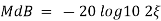
MdB = +20 log10
MdB = -20 log10
Decade frequency:
W present = 10  past
past
Then  present is called decade frequency of
  past
past
 2 = 10
  1
1
 2 is decade frequency of
  1
1
 MdB
MdB
0.01 40
0.1 20
1 0 (shows pole at origin)
0 -20
10 -40
100 -60
Slope = (20db/decade)
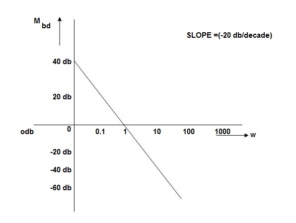
Fig 24 MAGNITUDE PLOT
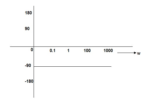
Fig 25 Phase Plot
Que. G(S) = 
Sol: G(j ) =
) = 
M =  ;
;  = -1800 (-20tan-1
 )
)
MdB = +20 log  -2
-2
MdB = -40 log10
 MdB
MdB
0.01 80
0.1 40
1 0 (pole at origin)
10 -40
100 -80
Slope = 40dbdecade
Que. G(S) = S
Sol: M= W
 = 900
= 900
MdB = 20 log10
 MdB
MdB
0.01 -40
0.1 -20
1 0
10 20
100 90
1000 60
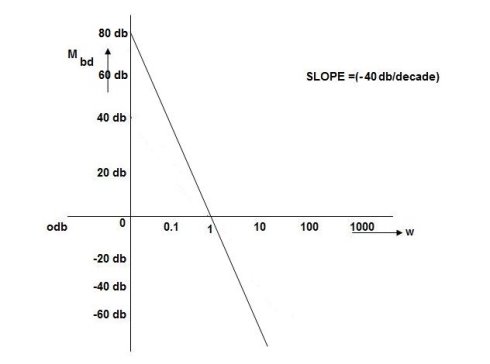
Fig 26 Bode Plot G(S) = S
Que. G(S) = S2
Sol: M=  2
2
MdB = 20 log10 2 = 40 log10
 = 1800
W MdB
0.01 -80
0.1 -40
1 0
10 40
100 80
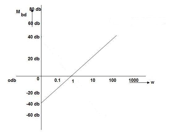
Fig 27 Magnitude Plot G(S) = S2
Que. G(S) = 
Sol: G(j ) =
) = 
M = 
MdB = 20 log10 K-20 log10
 = tan-1(
 ) –tan-1(
 )
)
 = 0-900 = -900
| K=1 |
| K=10 |
 | MDb |
| MdB |
| =-20 log10  | =20 -20 log10  |
|
0.01 | 40 |
| 60 |
0.1 | 20 |
| 40 |
1 | 0 |
| 20 |
10 | -20 |
| 0 |
100 | -40 |
| -20 |
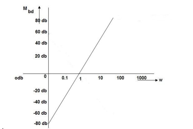
Fig 28 Bode Plot G(S) = 
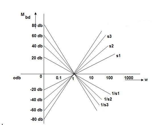
Fig 29 All bode plots in one plot
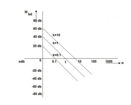
Fig 30 Variation in K shifts magnitude plot by +20db
As we vary K  then plot shift by 20 log10K i.e., adding a d.c. to a.c. Quantity
Approximation of Bode Plot:
If poles and zeros are not located at origin
G(S) = 
TF = 
M = 
MdB = -20 log10 (
 = -tan-1
Approximation:  T >> 1. So, we can neglect 1.
MdB = -20 log10
MdB = -20 log10 T.;
T.;  = -tan-1(
 T)
T)
Approximation:  T << 1. So, we can neglect
  T.
T.
MdB= 0dB,  = 00
= 00
At a point both meet so equal i.e., a time will come hence both approx. become equal
-20 log10 T= 0
T= 0
 T= 1
T= 1
 corner frequency
At this frequency both the cases are equal
MdB = -20 log10
Now for 
MdB = -20 log10
= -20 log10
= -10 log102
MdB = 10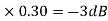
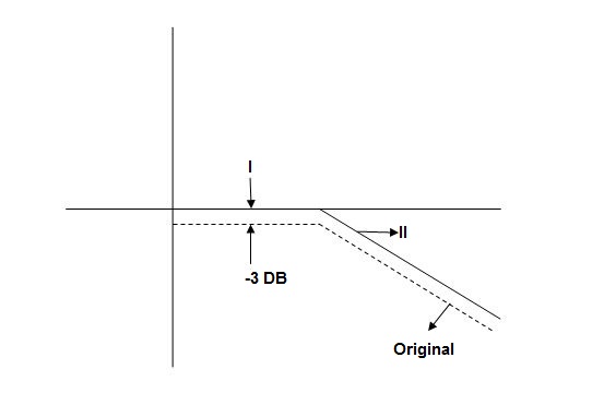
Fig 31 Approximation in bode plot
When we increase the value of  in app 2 and decrease the
  of app 1 so a RT comes when both cases are equal and hence for that value of
  where both app are equal gives max. Error we found above and is equal to 3dB
At corner frequency we have max error of -3Db
Que. G(S) = 
Sol: TF = 
M = 
MdB = -20 log10 ( at T=2
 MdB
MdB
1 -20 log10
10 -20 log10
100 -20 log10
 MdB
MdB  =
= =
= 
0.1 -20 log10 = 1.73
  10-3
10-3
0.1 -20 log10 = -0.1703
0.5 -20 log10 = -3dB
1 -20 log10 = -6.98
10 -20 log10 = -26.03
100 -20 log10 = -46.02
Fig 32 Magnitude Plot with approximation
Without approximation
For second order system
TF = 
TF = 
= 
= 
= 
M= 
MdB= 
Case 1  <<
<<
 << 1
<< 1
MdB= 20 log10 = 0 dB
Case 2  >>
>>
 >> 1
>> 1
MdB = -20 log10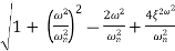
= -20 log10
= -20 log10
 < 1
< 1  is very large so neglecting other two terms
MdB = -20 log10
= -40 log10
Case 3. When case 1 is equal to case 2
-40 log10 = 0
= 0
 = 1
= 1

The natural frequency is our corner frequency
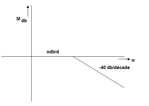
Fig 33 Magnitude Plot
Max error at  i. e at corner frequency
MdB = -20 log10
For 
MdB = -20 log10 
 error for
Completely the error depends upon the value of  (error at corner frequency)
The maximum error will be
MdB = -20 log10 
M = -20 log10 
 = 0
= 0

 is resonant frequency and at this frequency we are getting the maximum error so the magnitude will be
M = - +
+ 
= 
Mr =
MdB = -20 log10
MdB = -20 log10 
 = tan-1

Mr = 
Type of system | Initial slope | Intersection |
0 | 0 dB/decade | Parallel to 0 axis |
1 | -20 dB/decade | =K1 |
2 | -40 dB/decade | =K1/2 |
3 | -60 dB/decade | =K1/3 |
. | . | 1 |
. | . | 1 |
. | . | 1 |
N | -20N dB/decade | =K1/N |
Gain Cross Over Frequency
The frequency at which the bode plot culls the 0db axis is called as Gain Cross Over Frequency.
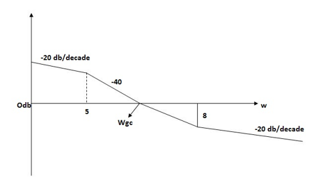
Fig 34 Gain cross over frequency
Phase Cross Over Frequency
The Frequency at which the phase plot culls the -1800 axis.
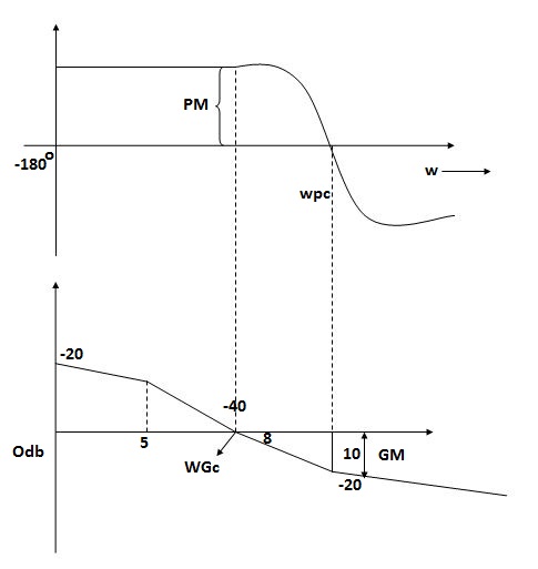
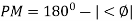
Fig 35 Phase Margin and Gain Margin
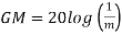
GM=MdB= -20 log [ G (jw)]
 .:
.: 
 .:
.: 
Key takeaway
i) More the difference b/WPC and WGC core are the stability of system
Ii) If GM is below 0dB axis than take +ve and stable. If GM above 0dB axis, that is take -ve
GM= ODB - 20 log M
Iii) The IM should also lie above -1800 for making the system (i.e., pm=+ve
Iv) For a stable system GM and PM should be -ve
v) GM and PM both should be +ve more the value of GM and PM more the system is stable.
Vi) If Wpc and Wgc are in same line Wpc= Wgc than system is marginally stable as we get GM=0dB.
Vii) When gain cross over frequency is smaller than phase curves over frequency the system is stable and vice versa.
The greater the Gain Margin (GM), the greater the stability of the system. The gain margin refers to the amount of gain, which can be increased or decreased without making the system unstable. It is usually expressed as a magnitude in dB.
We can usually read the gain margin directly from the Bode plot (as shown in the diagram above). This is done by calculating the vertical distance between the magnitude curve (on the Bode magnitude plot) and the x-axis at the frequency where the Bode phase plot = 180°. This point is known as the phase crossover frequency.
The greater the Phase Margin (PM), the greater will be the stability of the system. The phase margin refers to the amount of phase, which can be increased or decreased without making the system unstable. It is usually expressed as a phase in degrees.
We can usually read the phase margin directly from the Bode plot (as shown in the diagram above). This is done by calculating the vertical distance between the phase curve (on the Bode phase plot) and the x-axis at the frequency where the Bode magnitude plot = 0 dB. This point is known as the gain crossover frequency.
Sketch of Bode Plot
Q.1 Sketch the bode plot for transfer function
G(S) = 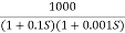
1. Replace S = j
G (j =
= 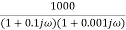
This is type 0 system. So initial slope is 0 dB decade. The starting point is given as
20 log10 K = 20 log10 1000
= 60 dB
Corner frequency  1 =
1 =  = 10 rad/sec
 2 =
2 =  = 1000 rad/sec
Slope after  1 will be -20 dB/decade till second corner frequency i.e.,
  2 after
  2 the slope will be -40 dB/decade (-20+(-20)) as there are poles
2. For phase plot
 = tan-1 0.1
 - tan-1 0.001
For phase plot


100 -900
200 -9.450
300 -104.80
400 -110.360
500 -115.420
600 -120.00
700 -124.170
800 -127.940
900 -131.350
1000 -134.420
The plot is shown in figure below
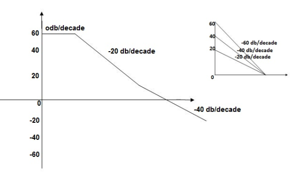
Fig 36 Magnitude Plot for G(S) = 
Q.2 For the given transfer function determine
G(S) = 
Gain cross over frequency phase cross over frequency phase mergence and gain margin
Initial slope = 1
N = 1, (K)1/N = 2
K = 2
Corner frequency
 1 =
1 =  = 2 (slope -20 dB/decade
 2 =
2 =  = 20 (slope -40 dB/decade

Phase
 = tan-1
 - tan-1 0.5
  - tan-1 0.05
 = 900- tan-1 0.5
  - tan-1 0.05


1 -119.430
5 -172.230
10 -195.250
15 -209.270
20 -219.30
25 -226.760
30 -232.490
35 -236.980
40 -240.570
45 -243.490
50 -245.910
Finding  gc (gain cross over frequency
M = 
4 =  2 (
2 ( (
(
 6 (6.25
 104) + 0.252
 4 +
4 + 2 = 4
2 = 4
Let  2 = x
2 = x
X3 (6.25 104) + 0.252
 2 + x = 4
X1 = 2.46
X2 = -399.9
X3 = -6.50
For x1 = 2.46
 gc = 3.99 rad/sec (from plot)
For phase margin
PM = 1800 - 
 = 900 – tan-1 (0.5×
 gc) – tan-1 (0.05 ×
  gc)
gc)
= -164.50
PM = 1800 - 164.50
= 15.50
For phase cross over frequency ( pc)
pc)
 = 900 – tan-1 (0.5
  ) – tan-1 (0.05
  )
)
-1800 = -900 – tan-1 (0.5  pc) – tan-1 (0.05
  pc)
pc)
-900 – tan-1 (0.5  pc) – tan-1 (0.05
  pc)
pc)
Taking than on both sides
Tan 900 = tan-1
Let tan-1 0.5  pc = A, tan-1 0.05
  pc = B
 = 00
= 00
 = 0
= 0
1 =0.5  pc 0.05
 pc
pc
 pc = 6.32 rad/sec
The plot is shown in figure below
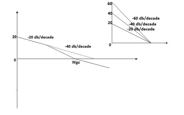 Fig 37 Magnitude Plot G(S) =
Q3. For the given transfer function
G(S) = 
Plot the rode plot find PM and GM
Sol: T1 = 0.5  1 =
1 =  = 2 rad/sec
Zero so, slope (20 dB/decade)
T2 = 0.2  2 =
2 =  = 5 rad/sec
Pole, so slope (-20 dB/decade)
T3 = 0.1 = T4 = 0.1
 3 =
3 =  4 = 10 (2 pole) (-40 db/decade)
1. Initial slope 0 dB/decade till  1 = 2 rad/sec
2. From  1 to
1 to 2 (i.e., 2 rad /sec to 5 rad/sec) slope will be 20 dB/decade
3. From  2 to
2 to  3 the slope will be 0 dB/decade (20 + (-20))
4. From  3,
3, 4 the slope will be -40 dB/decade (0-20-20)
Phase plot
 = tan-1 0.5
 - tan-1 0.2
 - tan-1 0.1
 - tan-1 0.1


500 -177.30
1000 -178.60
1500 -179.10
2000 -179.40
2500 -179.50
3000 -179.530
3500 -179.60
GM = 00
PM = 61.460
The plot is shown in figure below
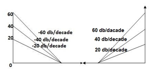
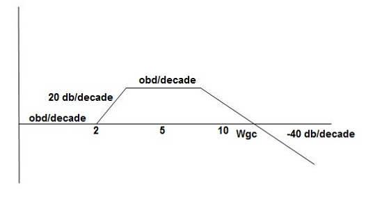
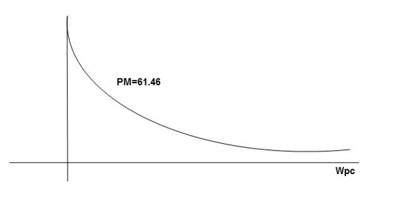
Fig 38 Magnitude and phase Plot for G(S) = 
Q 4. For the given transfer function plot the bode plot (magnitude plot) G(S) = 
Sol: Given transfer function
G(S) = 
Converting above transfer function to standard from
G(S) = 
= 
1. As type 1 system, so initial slope will be -20 dB/decade
2. Final slope will be -60 dB/decade as order of system decides the final slope
3. Corner frequency
T1 =  ,
,  11= 5 (zero)
T2 = 1,  2 = 1 (pole)
4. Initial slope will cut zero dB axis at
(K)1/N = 10
i.e.,  = 10
= 10
5. Finding  n and
n and 
T(S) = 
T(S)= 
Comparing with standard second order system equation
S2+2 ns +
ns + n2
n2
 n = 11 rad/sec
 n = 5
n = 5
 11 = 5
 =
=  = 0.27
6. Maximum error
M = -20 log 2
= +6.5 dB
As K = 10, so whole plot will shift by 20 log 10 10 = 20 dB
The plot is shown in figure below
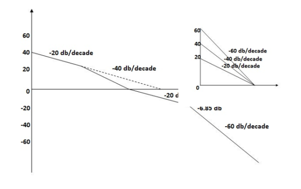
Fig 39 Magnitude Plot for G(S) = 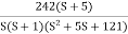
Q5. For the given plot determine the transfer function
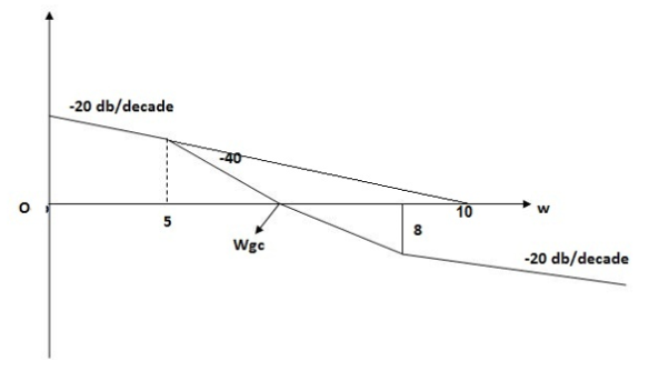
Fig 40 Magnitude Plot
Sol: From figure above, we can conclude that
1. Initial slope = -20 dB/decade so type -1
2. Initial slope all 0 dB axis at  = 10 so
K1/N N = 1
(K)1/N = 10.
3. Corner frequency
 1 =
1 =  = 0.2 rad/sec
 2 =
2 =  = 0.125 rad/sec
4. At  = 5 the slope becomes -40 dB/decade, so there is a pole at
  = 5 as slope changes from -20 dB/decade to -40 dB/decade
5. At  = 8 the slope changes from -40 dB/decade to -20 dB/decade hence is a zero at
  = 8 (-40+(+20) = 20)
6. Hence transfer function is T(S) = 
References:
- Alciatore & Histand, Introduction to Mechatronics and Measurement system, 4th Edition, Mc-Graw Hill publication, 2011
- Bishop (Editor), Mechatronics – An Introduction, CRC Press, 2006
- Mahalik, Mechatronics – Principles, concepts and applications, Tata Mc-Graw Hill publication, New Delhi
- C. D. Johnson, Process Control Instrumentation Technology, Prentice Hall, New Delhi


