UNIT – 3

Economics

3.1 THEORY OF DEMAND :

Theory of Demand

Theory of Demand is the principle/law that correlates the demand for a product with the price of the product. The Law of Demand is the basis for price determination in an open market.

3.2 LAW OF DEMAND :

The law of demand explains how the consumer’s choice-behaviour changes when there is a change in the price of a commodity. In a market situation , if other factors affecting demand for commodity does not change, but only the price changes, then a consumer is likely to buy more of a commodity when its price falls and less of a commodity when its price rises. This behaviour of a consumer is a commonly observed behaviour and the law of demand is based on such observed behaviour.

The law of demand, i.e., the inverse relationship between the price and the quantity demanded of a good, is explained through demand curve in Fig. 3.1.

In Fig.3.1. The price is measured on the vertical axis and quantity demanded on the horizontal axis. The lines DD is the demand curve. It slopes downwards from left to right. It shows the inverse relationship between the price and quantity demanded.

The Law of Demand is based on the following assumptions:

• No change in consumer’s income : During the operation of the law, the income of the consumer should remain the same. If income rises, the consumer may buy more at same price or buy the same quantity even if price rises.
• No changes in price of related goods : Prices of substitutes and complements should remain the same . It they change, the consumer’s preferences will change which may invalidate the law of demand .
• No change in taste : The term taste includes fashion, habits and other factors which influence consumer’s preferences. They should remain constant. If they change the demand will change at the existing price.
• No uncertainty about the future : If the consumers are uncertain about the future price, availability of goods and other economic and political factors, demand would change depending upon people’s expectations. For example, if consumers expect prices to rise and shortages in supply , they will purchase more at the same price  or even at a higher price. Such uncertainties are assumed not to be present.
• No change in the size of population and its composition : Market demand is affected by the size and composition of the population. Change in population and changes in sex and age composition will affect demand. An increase in population will increase the demand at the same price. Similarly an increase in number of children will increase demand for toys. Thus, size of population and its composition are assumed to remain constant.
• No change in advertisement : Effective and extensive advertisement of the product will affect consumers’ preferences. Thus, advertisement costs and efforts are assumed to remain constant.
• No change in government policy : Direct taxes on increase may reduce demand, while subsidies may increase the demand.
• No change in natural factors : Climates conditions are assumed to remain constant and have no effect on demand.   

The Law of demand, while explaining the relationship between price and quantity demanded, expects all factors other than the price to remain constant.

All the constant factors are put under the assumption “other things being equal “ (ceteris paribus), while explaining the law of demand.

Exceptions to Law of Demand :

The law of demand is not applicable in the following cases :

• Giffen goods : These are special types of inferior goods which are purchased more at a higher price and less at a lower price.
• Snob value : Rich consumers, who attach a snob value to owning and displaying expensive goods such a diamonds, jewellery ,etc. purchase more such goods as their prices rise. On the other hand, as their prices fall, the same consumers may buy less due to the loss of snob appeal because “everyone can afford them”.
• Price Expectations : When the prices are rising, consumers may purchase more of commodity if they expect prices will rise further. Similarly when the price falls, the consumers may not purchase more if they expect the price to fall further.
• Emergencies : In times of war, famine, major illness, etc.  households purchase more of the goods even when their price are rising.
• Fashion : When the consumers give importance to fashion, a rise in prices of these goods will not lower demand. Similarly, when a product goes out of fashion, a reduction in price of this product may not increase the demand for it. 

3.3 ELASTICITY OF DEMAND :

In general terms, we can define elasticity as the percentage change in one variable (for e.g. A ) to the percentage change in another variable (for e.g. B ). Thus,

Coefficient of elasticity =    =  ÷

The general concept of elasticity given above can be used to explain the following elasticities of demand.

1. Price elasticity of demand
2. Income elasticity of demand
3. Cross elasticity of demand
4. Promotional elasticity of demand

The above types of elasticity of demand show the degree of responsiveness of demand to a change in relevant determinants. In general terms, a coefficient of elasticity can be calculated for each of the above categories using the following general formula :

Coefficient of demand  elasticity =

PRICE ELASTICITY OF DEMAND

This measures the responsiveness of quantity demanded of commodity to a change in its price. The price elasticity of demand (Ep) is given by the percentage change in the quantity demanded of the commodity dividend by the percentage change in its price, keeping constant all other variables in the demand function. That is,

Ep =

Since the demand curve for most commodities, is downward sloping due to the inverse relationship between price and the quantity demanded of a commodity, the value of the price elasticity of demand will always be negative. However, while interpreting the price elasticity of demand the negative sign is ignored or omitted.

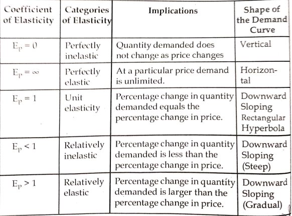
DIFFERENT DEGREES OF ELASTICITY :

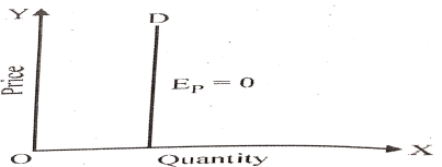
• Perfectly Inelastic Demand : Ep = 0   
• When the demand for a commodity is not responsive any change in price, demand is perfectly inelastic. In this case the demand curve will be a vertical line, as in Fig. And Ep is equal to zero at every point on this demand curve. Example : Insulin to a diabetic.

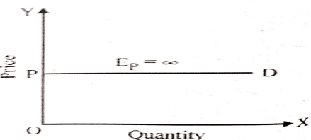
• Perfectly Elastic Demand : Ep = ∞

• Demand is perfectly elastic when consumer are prepared to buy all that is available in the market at a particular price. In this case the demand curve is horizontal at the given price OP, as in Fig. If price is increased, even marginally, nothing will be purchased.

This type of demand curve is relevant to perfect competition.

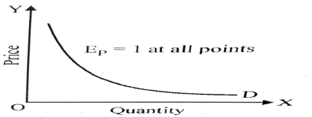
• Unity Elasticity of demand : Ep=1
• Demand is unitary elastic when the percentage change in quantity demanded equals the percentage change in price. In this case the demand curve is a rectangular hyperbola* as in Fig. At any point on the curve the value of elasticity is equal to unity.
• *Rectangular Hyperbola : The area under the demand curve is constant at all price-quantity combination. Such a demand curve represents constant TR (PXQ) in case of any change in price.

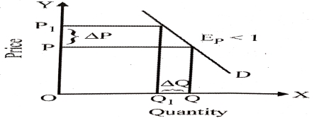
• Relatively Inelastic Demand : Ep<1

• Demand in relatively inelastic when the percentage change in quantity demanded is less than percentage change in price. In thi case the demand curve is steeper as in Fig. And therefore change in price (∆P) is greater than change in quantity demanded (∆Q) = ∆P > ∆Q.
• Examples : Essential commodities like petrol, diesel , commodities with few substitutes, like electricity, high-value luxury goods like sports cars.

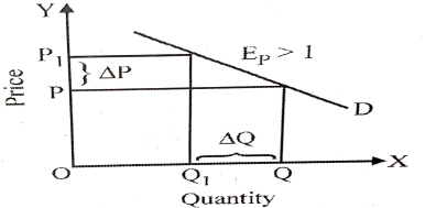
• Relatively Elastic Demand : Ep > 1

• Demand is relatively elastic when the percentage change in quantity demanded is greater than percentage change in price. In this case the demand curve is flatter as in Fig. And therefore ∆P < ∆Q.
• Examples : Most mid-range consumer durables like cars, T.V.s, air conditioner , commodities with several substitutes like unbranded garments.

These different degree of price elasticity.

INCOME ELASTICITY OF DEMAND

The measures the responsiveness of demand for a commodity to a commodity to a change in consumer’s income. The income elasticity of demand (Ey) is given by the percentage change in income, keeping constant all other variables, including price in the demand function .

Ey =

As with price elasticity, income elasticity can be found out by point or arc method. Point income elasticity of demand is given by

Ey = = •

Where, ∆Q = Change in quantity demanded

∆Y = Change in income

Q = Original quantity demanded

Y = Original income

CROSS ELASTICITY OF DEMAND

Price elasticity of demand for a commodity explains the changes in quantity demanded due to change in the price of the commodity. Demand for a commodity may change not only due to a change in its own price but due to the change in the price of  a substitute or complementary commodity. A change in demand for a commodity due to a change in the price of its substitute or complementary good is termed cross elasticity of demand. For example, if the price of Pepsi rises, Consumers may switch over to coke, assuming that there is no change in the price of coke .

Cross elasticity of demand (Ec) measures the responsiveness in the demand for commodity X to a change in the price of commodity Y. It is given by the percentage change in the quantity demanded for commodity X dividend by the percentage change in the price of commodity Y, keeping constant all other variables in the demand function. Thus,

Ec =

3.4 CONSUMER SURPLUS:

The concept of consumer surplus is derived from the law of diminishing marginal utility. As per the law, as we purchase more of a commodity, its marginal utility reduces. Since the price is fixed, for all units of the goods we purchase, we get extra utility. This extra utility is consumer surplus.

Consumer Surplus

Alfred Marshall, British Economist defines consumer’s surplus as follows: “Excess of the price that a consumer would be willing to pay rather than go without a commodity over that which he actually pays.”

Hence, Consumer’s Surplus = The price a consumer is ready to pay – The price he actually pays

Further, the consumer is in equilibrium when the marginal utility is equal to the price. That is, he purchases those many numbers of units of a good at which the marginal utility is equal to the price. Now, the price is fixed for all units. Hence, he gets a surplus for all units except the one at the margin. This extra utility is consumer surplus.

Let us take a look at an example of consumer surplus.

No. Of units Marginal Utility Price (Rs.) Consumer’s Surplus

1   30   20   10

2   28   20   8

3   26   20   6

4   24   20   4

5   22   20   2

6   20   20   0

7   18   20   –

From the table above, we see that as the consumption increase from 1 to 2 units, the marginal utility falls from 30 to 28. This diminishes further as he increases consumption. Now,

Marginal utility is the price the consumer is willing to pay for that unit.

The actual price of the unit is fixed.

Therefore, the consumer enjoys a surplus on all purchases until the sixth unit. When he buys the sixth unit, he is in equilibrium, since the price he is willing to pay is equal to the actual price of the unit.

Limitations

It is difficult to measure the marginal utilities of different units of a commodity consumed by a person. Hence, the precise measurement of consumer’s surplus is not possible.

For necessary goods, the marginal utilities of the first few units are infinitely large. Hence the consumer’s surplus is infinite for such goods.

The availability of substitutes also affects the consumer’s surplus.

Deriving the utility scale for prestigious goods like diamonds is very difficult.

We cannot measure the consumer’s surplus in terms of money. This is because the marginal utility of money changes as a consumer makes purchases and his stock of money diminishes.

This concept is acceptable only on the assumption that we can measure utility in terms of money or otherwise. Many modern economists are against the concept.

3.5 INDIFFERENCE CURVE:

What is an Indifference Curve?

It is a curve that represents all the combinations of goods that give the same satisfaction to the consumer. Since all the combinations give the same amount of satisfaction, the consumer prefers them equally. Hence the name Indifference Curve.

Here is an example to understand the indifference curve better. Peter has 1 unit of food and 12 units of clothing. Now, we ask Peter how many units of clothing is he willing to give up in exchange for an additional unit of food so that his level of satisfaction remains unchanged.

Peter agrees to give up 6 units of clothing for an additional unit of food. Hence, we have two combinations of food and clothing giving equal satisfaction to Peter as follows:

1 unit of food and 12 units of clothing

2 units of food and 6 units of clothing

By asking him similar questions, we get various combinations as follows:

Combination Food Clothing

A         1 12

B   2 6

C   3 4

D   4 3

The diagram shows an Indifference curve (IC). Any combination lying on this curve gives the same level of consumer satisfaction. It is also known as Iso-Utility Curve.

3.6 PRODUCTION-LAW OF RETURNS:

Laws of returns to scale refers to the long-run analysis of the laws of production. In the long run output can be increased by varying all factors. Thus, in this section we study the change in output as a result of change in all factors. In other words, we study the behaviour of output in response to change in the scale. When all factors are increased in the same proportion an increase in scale occurs.

Scale refers to quantity of all factors which re employed in optimal combinations for specified outputs. The terms ‘returns to scale’ refers to the degree by which output changes as a result of a given change in the quantity of all inputs used in production. We have three types of returns to scale: constant, increasing and decreasing. If output increases by the same proportion s the increases more than proportionally with the increase in inputs, we have increasing returns to scale. If output increases less than proportionally with the increases in inputs we have decreasing returns to scale. Thus, returns to scale may be constant, increasing or decreasing depending upon whether output increases in the same, greater or lower rate in response to a proportionate increase in all inputs. Returns to scale can be expressed as a movement along the scale line or expansion path which we have seen in the previous section. The three types of returns to scale are explained below.

Constant Returns to Scale

If outputs increase in the same proportion as the increase in inputs, returns to scale are said to be constant.  Thus, doubling of all factor inputs causes doubling of  the level of outputs; trebling of inputs causes trebling of outputs, and so on. The case of constant returns to scale is sometimes called linear homogenous production function. This is illustrated with the help of isoquants in fig. Where the line OE is the scale line. The scale line indicates the increase in scale. It can be observed from fig. That the distance between successive isoquants is equal, that is, Oa=ab=bc. It means that if both labour and capital are increased in a given proportion the output expands in the same proportion as the numbers 100,200 and 300 against the isoquants indicate.

Increasing Returns to Scale       

When the output increases at  a greater proportion  than the increase in inputs, returns to scale are said to be increasing. It is explained in fig. When the returns to scale are increasing the distance between successive isoquants becomes less and less, that is Oa>ab>bc. It means tht equal increases in output, i.e. 100 unit at each isoquants are obtained by smaller and smaller increments in inputs. In other words, by doubling inputs the output is more doubled.

Increasing returns to scale arise on account of indivisibilities of some factors. As output is increased the indivisible factors are better utilized and therefore, increasing returns to scale arise. In other words, the returns to scale are increasing due to economies of scale.

Decreasing Returns to Scale          

When the output increases in a smaller proportion than the increase in all inputs returns to scale re said to be decreasing. It is explained in fig.

It can be seen from fig. That the distance between successive isoquants are increasing, that is, Oa<ab<bc. It means that equal increments that is 100 units, in output are obtained by larger and larger increases in inputs. In other words, if the inputs are doubled, output will increase by less than twice its original level. The decreasing returns to scale are caused by diseconomies of large scale production.

3.7 ISO-PRODUCTIVE CURVE:

MEANING  

An iso-product curve is locus of various combinations of two factors of production giving the same level of output and a producer is indifferent to each of such combinations. All the combinations of two inputs give the same quantum of output to a producer and the producer is indifferent to each such combination. He does not have any preference. These iso-product curves are also called production indifference curves. The concept of iso-product curve can be explained with the help of iso-quant schedule and diagram.

Iso-Quant Schedule:

An iso-quant schedule shows different combinations of two factors of production (inputs) at which a producer gets equal quantum of output.

3.8 NATURE OF COSTS, FIXED COSTS, VARIABLES COST, TOTAL, AVERAGE AND MARGINAL COSTS:

INTRODUCTION

A profit maximizing firm needs to monitor continuously about its cost and revenue. It is level of cost relative to revenue that determines the overall profitability of the firm. In order to maximise profits a firm has to increase its revenue and lower its cost.

Money Cost – Implicit and Explicit 

Implicit costs (IC) are due to the factors which the entrepreneur himself oens and employs in the firm.

Explicit costs (EC) are the contractual cash payments made by the firm for purchasing or hiding the various factors.

Fixed, Variable and Total Cost

Fixed Cost

Total cost of production consists of fixed cost and variable cost.

Fixed costs are those which is independent of output. They must be paid even if the firm produces no output. They will not change even if output changes. They remain fixed whether output is large or small. Fixed costs are also called “overhead costs” or “supplementary costs”. They include such payments as rents, interest, insurance, depreciation charges maintenance costs, property taxes, administrative expense like manager’s salary and so on.               

Variable Cost

Variable cost are those which are incurred on the employment of variable factors of production. They vary with the level of output. They increase with rise in output and decrease with the fall in output. By definition variable costs remain zero when output is zero. They include payments for wages, raw materials, fuel, power, transport and the like. Marshall called these variable costs as “Prime Costs” of production.

Average Total Cost (ATC)

One of the most important cost concept is average total cost. It, when compared with price or average revenue, will allow a business to determine whether or not it is making a profit. Average total cost is total cost divided by the number of unts produced i.e.

Average Total Cost = = =ATC

Where q represents the number of units of output produced.

Marginal Cost (MC)

Marginal Cost is the extra or additional cost of producing on extra unit of output. In economics the term ‘marginal’ whether applied to utility, cost, production, consumption or whatever, means ‘incremental’ or ‘extra’. Thus, marginal cost is the cost is the total cost of n units of output minus the total cost of n-1 units. In symbols:

MCn = TCn – TCn-1