UNIT 5
Correlation
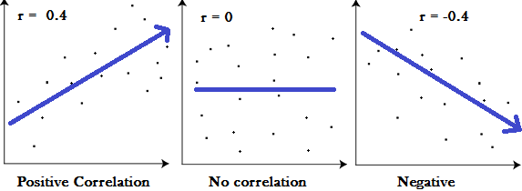
Correlation measures the nature and strength of relationship between two variables. Correlation lies between +1 to -1. A correlation of +1 indicates a perfect positive correlation between two variables. A zero correlation indicates that there is no relationship between the variables. A correlation of -1 indicates a perfect negative correlation.
Definition
“Correlation analysis deals with the association between two or more variables.” —Simpson and Kafka
“Correlation is an analysis of the co-variation between two variables.” —A.M. Tuttle
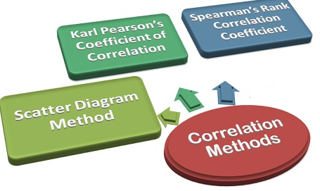
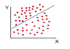
- Scatter diagram method is the simplest method to study correlation between two variables. The correlations of two variables are plotted in the graph in the form of dots thereby obtaining as many points as the number of observations. The degree of correlation is ascertained by looking at the scattered points over the charts.
The more the points plotted are scattered over the chart, the lesser is the degree of correlation between the variables. The more the points plotted are closer to the line, the higher is the degree of correlation. The degree of correlation is denoted by “r”.
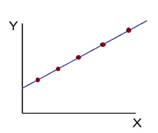
- Perfect positive correlation (r = +1) – All the points plotted on the straight line rising from left to right
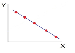
- Perfect negative correlation (r=-1) – all the points plotted on the straight line falling from left to right
- High Degree of +Ve Correlation (r= + High): all the points plotted close to the straight line rising from left to right
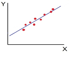
- High Degree of –Ve Correlation (r= – High) - all the points plotted close to the straight line falling from left to right.
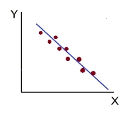
- Low degree of +Ve Correlation (r= + Low): all the points are highly scattered to the straight line rising from left to right
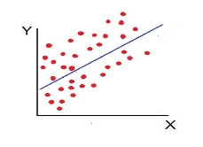
- Low Degree of –Ve Correlation (r= - Low): all the points are highly scattered to the straight line falling from left to right
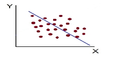
- No Correlation (r= 0) – all the points are scattered over the graph and do not show any pattern
2. Karl Pearson’s Coefficient of Correlation is widely used mathematical method is used to calculate the degree and direction of the relationship between linear related variables. The coefficient of correlation is denoted by “r”.
Direct method
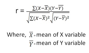
Shortcut method –


The value of the coefficient of correlation (r) always lies between ±1. Such as:
- r=+1, perfect positive correlation
- r=-1, perfect negative correlation
- r=0, no correlation
Example 1 - Compute Pearsons coefficient of correlation between advertisement cost and sales as per the data given below:
Advertisement cost | 39 | 65 | 62 | 90 | 82 | 75 | 25 | 98 | 36 | 78 |
Sales | 47 | 53 | 58 | 86 | 62 | 68 | 60 | 91 | 51 | 84 |
Solution
X | Y |
|
|
|
|
 |
39 | 47 | -26 | 676 | -19 | 361 | 494 |
65 | 53 | 0 | 0 | -13 | 169 | 0 |
62 | 58 | -3 | 9 | -8 | 64 | 24 |
90 | 86 | 25 | 625 | 20 | 400 | 500 |
82 | 62 | 17 | 289 | -4 | 16 | -68 |
75 | 68 | 10 | 100 | 2 | 4 | 20 |
25 | 60 | -40 | 1600 | -6 | 36 | 240 |
98 | 91 | 33 | 1089 | 25 | 625 | 825 |
36 | 51 | -29 | 841 | -15 | 225 | 435 |
78 | 84 | 13 | 169 | 18 | 324 | 234 |
650 | 660 |
| 5398 |
| 2224 | 2704 |
|
|
|
|
|
|
|

r = (2704)/√5398 √2224 = (2704)/(73.2*47.15) = 0.78
Thus Correlation coefficient is positively correlated
Example 2
Compute correlation coefficient from the following data
Hours of sleep (X) | Test scores (Y) |
8 | 81 |
8 | 80 |
6 | 75 |
5 | 65 |
7 | 91 |
6 | 80 |
X | Y |
|
|
|
|
 |
8 | 81 | 1.3 | 1.8 | 2.3 | 5.4 | 3.1 |
8 | 80 | 1.3 | 1.8 | 1.3 | 1.8 | 1.8 |
6 | 75 | -0.7 | 0.4 | -3.7 | 13.4 | 2.4 |
5 | 65 | -1.7 | 2.8 | -13.7 | 186.8 | 22.8 |
7 | 91 | 0.3 | 0.1 | 12.3 | 152.1 | 4.1 |
6 | 80 | -0.7 | 0.4 | 1.3 | 1.8 | -0.9 |
40 | 472 |
| 7 |
| 361 | 33 |

X = 40/6 =6.7

Y = 472/6 = 78.7

r = (33)/√7 √361 = (33)/(2.64*19) = 0.66
Thus Correlation coefficient is positively correlated
Example 3
Calculate coefficient of correlation between X and Y series using Karl pearson shortcut method
X | 14 | 12 | 14 | 16 | 16 | 17 | 16 | 15 |
Y | 13 | 11 | 10 | 15 | 15 | 9 | 14 | 17 |
Solution
Let assumed mean for X = 15, assumed mean for Y = 14
X | Y | Dx | Dx2 | Dy | Dy2 | Dxdy |
14 | 13 | -1.0 | 1.0 | -1.0 | 1.0 | 1.0 |
12 | 11 | -3.0 | 9.0 | -3.0 | 9.0 | 9.0 |
14 | 10 | -1.0 | 1.0 | -4.0 | 16.0 | 4.0 |
16 | 15 | 1.0 | 1.0 | 1.0 | 1.0 | 1.0 |
16 | 15 | 1.0 | 1.0 | 1.0 | 1.0 | 1.0 |
17 | 9 | 2.0 | 4.0 | -5.0 | 25.0 | -10.0 |
16 | 14 | 1 | 1 | 0 | 0 | 0 |
15 | 17 | 0 | 0 | 3 | 9 | 0 |
120 | 104 | 0 | 18 | -8 | 62 | 6 |

 r = 8 *6 – (0)*(-8)
√8*18-(0)2 √8*62 – (-8)2
r = 48/√144*√432 = 0.19
Example 4 - Calculate coefficient of correlation between X and Y series using Karl pearson shortcut method
X | 1800 | 1900 | 2000 | 2100 | 2200 | 2300 | 2400 | 2500 | 2600 |
F | 5 | 5 | 6 | 9 | 7 | 8 | 6 | 8 | 9 |
Solution
Assumed mean of X and Y is 2200, 6
X | Y | Dx | Dx (i=100) | Dx2 | Dy | Dy2 | Dxdy |
1800 | 5 | -400 | -4 | 16 | -1.0 | 1.0 | 4.0 |
1900 | 5 | -300 | -3 | 9 | -1.0 | 1.0 | 3.0 |
2000 | 6 | -200 | -2 | 4 | 0.0 | 0.0 | 0.0 |
2100 | 9 | -100 | -1 | 1 | 3.0 | 9.0 | -3.0 |
2200 | 7 | 0 | 0 | 0 | 1.0 | 1.0 | 0.0 |
2300 | 8 | 100 | 1 | 1 | 2.0 | 4.0 | 2.0 |
2400 | 6 | 200 | 2 | 4 | 0 | 0 | 0.0 |
2500 | 8 | 300 | 3 | 9 | 2 | 4 | 6.0 |
2600 | 9 | 400 | 4 | 16 | 3 | 9 | 12.0 |
|
|
|
|
|
|
|
|
|
|
| 0 | 60 | 9 | 29 | 24 |
Note – we can also proceed dividing x/100
 r = (9)(24) – (0)(9)
√9*60-(0)2 √9*29– (9)2
r = 0.69
Example 5 –
X | 28 | 45 | 40 | 38 | 35 | 33 | 40 | 32 | 36 | 33 |
Y | 23 | 34 | 33 | 34 | 30 | 26 | 28 | 31 | 36 | 35 |
Solution
X | Y |
|
|
|
|
 |
28 | 23 | -8 | 64 | -8.0 | 64.0 | 64.0 |
45 | 34 | 9 | 81 | 3.0 | 9.0 | 27.0 |
40 | 33 | 4 | 16 | 2.0 | 4.0 | 8.0 |
38 | 34 | 2 | 4 | 3.0 | 9.0 | 6.0 |
35 | 30 | -1 | 1 | -1.0 | 1.0 | 1.0 |
33 | 26 | -3 | 9 | -5.0 | 25.0 | 15.0 |
40 | 28 | 4 | 16 | -3 | 9 | -12.0 |
32 | 31 | -4 | 16 | 0 | 0 | 0.0 |
36 | 36 | 0 | 0 | 5 | 25 | 0.0 |
33 | 35 | -3 | 9 | 4 | 16 | -12 |
360 | 310 | 0 | 216 | 0 | 162 | 97 |

 X = 360/10 = 36
Y = 310/10 = 31

r = 97/(√216 √162 = 0.51
3. Spearman’s Rank Correlation Coefficient - The Spearman’s Rank Correlation Coefficient is the non-parametric statistical measure used to study the strength of association between the two ranked variables. This method is used for ordinal set of numbers, which can be arranged in order.

Where, P = Rank coefficient of correlation
D = Difference of ranks
N = Number of Observations
The Spearman’s Rank Correlation coefficient lies between +1 to -1.
- +1 indicates perfect association of rank
- 0 indicates no association between the rank
- -1 indicates perfect negative association between the ranks
When ranks are not given - Rank by taking the highest value or the lowest value as 1
Equal Ranks or Tie in Ranks – in this case ranks are assigned on an average basis. For ex – if three students score of 5, at 5th, 6th, 7th ranks ach one of them will be assigned a rank of 5 + 6 + 7/3= 6.
If two individual ranked equal at third position, then the rank is calculates as (3+4)/2 = 3.5
Example 1 –
Test 1 | 8 | 7 | 9 | 5 | 1 |
Test 2 | 10 | 8 | 7 | 4 | 5 |
Solution
Here, highest value is taken as 1
Test 1 | Test 2 | Rank T1 | Rank T2 | d | d2 |
8 | 10 | 2 | 1 | 1 | 1 |
7 | 8 | 3 | 2 | 1 | 1 |
9 | 7 | 1 | 3 | -2 | 4 |
5 | 4 | 4 | 5 | -1 | 1 |
1 | 5 | 5 | 4 | 1 | 1 |
|
|
|
|
| 8 |

R = 1 – (6*8)/5(52 – 1) = 0.60
Example 2 -
Calculate Spearman rank-order correlation
English | 56 | 75 | 45 | 71 | 62 | 64 | 58 | 80 | 76 | 61 |
Maths | 66 | 70 | 40 | 60 | 65 | 56 | 59 | 77 | 67 | 63 |
Solution
Rank by taking the highest value or the lowest value as 1.
Here, highest value is taken as 1
English | Maths | Rank (English) | Rank (Math) | d | d2 |
56 | 66 | 9 | 4 | 5 | 25 |
75 | 70 | 3 | 2 | 1 | 1 |
45 | 40 | 10 | 10 | 0 | 0 |
71 | 60 | 4 | 7 | -3 | 9 |
62 | 65 | 6 | 5 | 1 | 1 |
64 | 56 | 5 | 9 | -4 | 16 |
58 | 59 | 8 | 8 | 0 | 0 |
80 | 77 | 1 | 1 | 0 | 0 |
76 | 67 | 2 | 3 | -1 | 1 |
61 | 63 | 7 | 6 | 1 | 1 |
|
|
|
|
| 54 |

 R = 1-(6*54)
10(102-1)
R = 0.67
There fore this indicates a strong positive relationship between the ranks individuals obtained in the math and English exam.
Example 3 –
Find Spearman's rank correlation coefficient between X and Y for this set of data:
X | 13 | 20 | 22 | 18 | 19 | 11 | 10 | 15 |
Y | 17 | 19 | 23 | 16 | 20 | 10 | 11 | 18 |
Solution
X | Y | Rank X | Rank Y | d | d2 |
13 | 17 | 3 | 4 | -1 | 1 |
20 | 19 | 7 | 6 | 1 | 1 |
22 | 23 | 8 | 8 | 0 | 0 |
18 | 16 | 5 | 3 | 2 | 2 |
19 | 20 | 6 | 7 | -1 | 1 |
11 | 10 | 2 | 1 | 1 | 1 |
10 | 11 | 1 | 2 | -1 | 1 |
15 | 18 | 4 | 5 | -1 | 1 |
|
|
|
|
| 8 |
R =

 R = 1 – 6*8/8(82 – 1) = 1 – 48 = 0.90
504
Example 4 – calculation of equal ranks or tie ranks
Find Spearman's rank correlation coefficient:
Commerce | 15 | 20 | 28 | 12 | 40 | 60 | 20 | 80 |
Science | 40 | 30 | 50 | 30 | 20 | 10 | 30 | 60 |
Solution
C | S | Rank C | Rank S | d | d2 |
15 | 40 | 2 | 6 | -4 | 16 |
20 | 30 | 3.5 | 4 | -0.5 | 0.25 |
28 | 50 | 5 | 7 | -2 | 4 |
12 | 30 | 1 | 4 | -3 | 9 |
40 | 20 | 6 | 2 | 4 | 16 |
60 | 10 | 7 | 1 | 6 | 36 |
20 | 30 | 3.5 | 4 | -0.5 | 0.25 |
80 | 60 | 8 | 8 | 0 | 0 |
|
|
|
|
| 81.5 |

R = 1 – (6*81.5)/8(82 – 1) = 0.02
Example 5 –
X | 10 | 15 | 11 | 14 | 16 | 20 | 10 | 8 | 7 | 9 |
Y | 16 | 16 | 24 | 18 | 22 | 24 | 14 | 10 | 12 | 14 |
Solution
X | Y | Rank X | Rank Y | d | d2 |
10 | 16 | 6.5 | 5.5 | 1 | 1 |
15 | 16 | 3 | 5.5 | -2.5 | 6.25 |
11 | 24 | 5 | 1.5 | 3.5 | 12.25 |
14 | 18 | 4 | 4 | 0 | 0 |
16 | 22 | 2 | 3 | -1 | 1 |
20 | 24 | 1 | 1.5 | -0.5 | 0.25 |
10 | 14 | 6.5 | 7.5 | -1 | 1 |
8 | 10 | 9 | 10 | -1 | 1 |
7 | 12 | 10 | 9 | 1 | 1 |
9 | 14 | 8 | 7.5 | 0.5 | 0.25 |
|
|
|
|
| 24 |

R = 1 – (6*24)/10(102 – 1) = 0.85
The correlation between X and Y is positive and very high.
Sources
- B.N Gupta – Statistics
- S.P Singh – statistics
- Gupta and Kapoor – Statistics
- Yule and Kendall – Statistics method


