Unit - 1

Economics Theory

1.1 Features of Micro Economics:

• Unit of study: According to K.E. Boulding micro economics is the study of individual unit. It focuses attention on the study of the behavior of Micro variable. Thus, it studies only part of the economy and not the whole.
• Method: Micro economics is not concerned with the aggregate. What it really does is to slice (divide) the whole economy into smaller individual unit. So, economists point out that micro economics uses the Slicing method.
• Price theory: Micro economics analysis how the price of individual commodities and services are determined. Micro economics tells us how the price of individual commodity is decided, how the equilibrium of an individual firm reached etc. This is known as Price theory.             
• Area of Study: The main area of its study is the theory of product and factor pricing and their reaction to changes in demand and supply condition. Micro economics analyses the markets for the factors of production, that is, labour, capital, land and entrepreneur.
• Vision: Micro economics studies a small part of the economics through partial equilibrium. It studies in detail about behaviour of individual economics unit.  Micro economics studies how efficiently the various resources are allocated to individual consumers and producers within the economy. i.e. it examines the tree not the forest.
• Analysis allocation of resources: Micro economics analyses how resources are allocated to production of particular goods and services in the economy. Allocation of resources involves what to produce, how to produce and how much to produce. It also studies how efficiently the various resources are allocated to individual consumers and produces.
• Undertakes general equilibrium analysis: It is generally understood that micro economics does not concern itself with the economy as whole. But this is not correct. Micro economics examines the economy as a whole, but microscopically.
• Analysis of market structures: Micro Economics analyses different market structures i.e. perfect competition, monopoly, Oligopoly, monopolistic competition etc. and describes how prices and quantities are determined different markets.
• Limited scope: Micro Economics studies individual economic units & not the whole economy. It does not deal with the nation-wide problems like unemployment, inflation, deflation, poverty, balance of payment situation, economic growth etc. So its scope is limited.

1.2 Features of Macro economics:-

• Study of aggregates: Macro economics is a study of the aggregates. It is also known as aggregates economics. It studies the economics system as a whole covering all condition of the economy such as total production, total consumption, total saving and total investment. In the words of Prof. Mc connel, “Macro economics examines the forest, not the tree.”
• Lumping method: Macro economics deals with macro quantities and macro variable. Unlike macro economics, it does not split up the economy into small slice but studies in big lumps. Therefore it is called the method of lumping.
• General Equilibrium: Macroeconomic is based on general equilibrium. Whole economy is called general equilibrium. The technique of general equilibrium is applied to study the determination of the general price level, total employment and output.
• Vision: It gives the overall view of the whole economy i.e. it give a bird’s eye view of the whole economy.
• Interdependence: Macro analysis stresses interrelationship between the different Market and sectors in the economy. According to general equilibrium analysis, a change in any one market or sector will have its impact on the other markets or sectors of the economy.
• Income theory: Macro economics is known as income theory. It studies the factors determining national income and employment and the causes of fluctuations in income and employment. According to Edward Shapiro, the major task of macro economics is the explanation of what determines the economy’s income.
• Policy-oriented: Macro economics, according to Keynes’ is a policy-oriented science. Macro-economic analysis helps in formulating suitable economic policies to promote economic growth, to generate employment, to control inflation, to pull the economy out of depression etc.

The law of demand explains how the consumer’s choice-behaviour changes when there is a change in the price of a commodity. In a market situation , if other factors affecting demand for commodity does not change, but only the price changes, then a consumer is likely to buy more of a commodity when its price falls and less of a commodity when its price rises. This behaviour of a consumer is a commonly observed behaviour and the law of demand is based on such observed behaviour.

The law of demand, i.e., the inverse relationship between the price and the quantity demanded of a good, is explained through demand curve in Fig. 3.1.

In Fig.3.1. The price is measured on the vertical axis and quantity demanded on the horizontal axis. The lines DD is the demand curve. It slopes downwards from left to right. It shows the inverse relationship between the price and quantity demanded.

1.3 The Law of Demand is based on the following assumptions:

• No change in consumer’s income : During the operation of the law, the income of the consumer should remain the same. If income rises, the consumer may buy more at same price or buy the same quantity even if price rises.
• No changes in price of related goods : Prices of substitutes and complements should remain the same . It they change, the consumer’s preferences will change which may invalidate the law of demand .
• No change in taste : The term taste includes fashion, habits and other factors which influence consumer’s preferences. They should remain constant. If they change the demand will change at the existing price.
• No uncertainty about the future : If the consumers are uncertain about the future price, availability of goods and other economic and political factors, demand would change depending upon people’s expectations. For example, if consumers expect prices to rise and shortages in supply , they will purchase more at the same price  or even at a higher price. Such uncertainties are assumed not to be present.
• No change in the size of population and its composition : Market demand is affected by the size and composition of the population. Change in population and changes in sex and age composition will affect demand. An increase in population will increase the demand at the same price. Similarly an increase in number of children will increase demand for toys. Thus, size of population and its composition are assumed to remain constant.
• No change in advertisement : Effective and extensive advertisement of the product will affect consumers’ preferences. Thus, advertisement costs and efforts are assumed to remain constant.
• No change in government policy : Direct taxes on increase may reduce demand, while subsidies may increase the demand.
• No change in natural factors : Climates conditions are assumed to remain constant and have no effect on demand.   

The Law of demand, while explaining the relationship between price and quantity demanded, expects all factors other than the price to remain constant.

All the constant factors are put under the assumption “other things being equal “ (ceteris paribus), while explaining the law of demand.

1.4 Exceptions to Law of Demand :

The law of demand is not applicable in the following cases :

• Giffen goods : These are special types of inferior goods which are purchased more at a higher price and less at a lower price.
• Snob value : Rich consumers, who attach a snob value to owning and displaying expensive goods such a diamonds, jewellery ,etc. purchase more such goods as their prices rise. On the other hand, as their prices fall, the same consumers may buy less due to the loss of snob appeal because “everyone can afford them”.
• Price Expectations : When the prices are rising, consumers may purchase more of commodity if they expect prices will rise further. Similarly when the price falls, the consumers may not purchase more if they expect the price to fall further.
• Emergencies : In times of war, famine, major illness, etc.  households purchase more of the goods even when their price are rising.
• Fashion : When the consumers give importance to fashion, a rise in prices of these goods will not lower demand. Similarly, when a product goes out of fashion, a reduction in price of this product may not increase the demand for it. 

1.5 ELASTICITY

In general terms, we can define elasticity as the percentage change in one variable (for e.g. A ) to the percentage change in another variable (for e.g. B ). Thus,

Coefficient of elasticity =    =  ÷

The general concept of elasticity given above can be used to explain the following elasticities of demand.

1. Price elasticity of demand
2. Income elasticity of demand
3. Cross elasticity of demand
4. Promotional elasticity of demand

The above types of elasticity of demand show the degree of responsiveness of demand to a change in relevant determinants. In general terms, a coefficient of elasticity can be calculated for each of the above categories using the following general formula :

Coefficient of demand  elasticity =

1.6 PRICE ELASTICITY OF DEMAND

This measures the responsiveness of quantity demanded of commodity to a change in its price. The price elasticity of demand (Ep) is given by the percentage change in the quantity demanded of the commodity dividend by the percentage change in its price, keeping constant all other variables in the demand function. That is,

Ep =

Since the demand curve for most commodities, is downward sloping due to the inverse relationship between price and the quantity demanded of a commodity, the value of the price elasticity of demand will always be negative. However, while interpreting the price elasticity of demand the negative sign is ignored or omitted.

1.7 DIFFERENT DEGREES OF ELASTICITY :

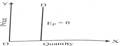
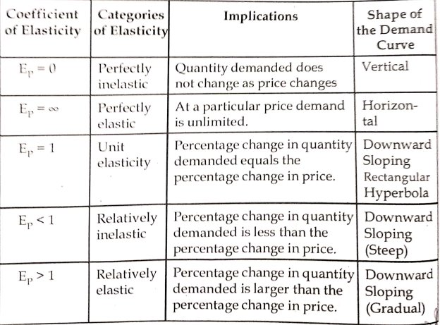
• Perfectly Inelastic Demand : Ep = 0   
• When the demand for a commodity is not responsive any change in price, demand is perfectly inelastic. In this case the demand curve will be a vertical line, as in Fig. And Ep is equal to zero at every point on this demand curve. Example : Insulin to a diabetic.

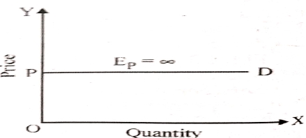
• Perfectly Elastic Demand : Ep = ∞

• Demand is perfectly elastic when consumer are prepared to buy all that is available in the market at a particular price. In this case the demand curve is horizontal at the given price OP, as in Fig. If price is increased, even marginally, nothing will be purchased.

This type of demand curve is relevant to perfect competition.

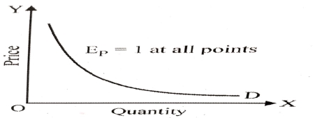
• Unity Elasticity of demand : Ep=1
• Demand is unitary elastic when the percentage change in quantity demanded equals the percentage change in price. In this case the demand curve is a rectangular hyperbola* as in Fig. At any point on the curve the value of elasticity is equal to unity.
• *Rectangular Hyperbola : The area under the demand curve is constant at all price-quantity combination. Such a demand curve represents constant TR (PXQ) in case of any change in price.

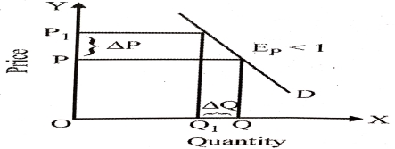
• Relatively Inelastic Demand : Ep<1

• Demand in relatively inelastic when the percentage change in quantity demanded is less than percentage change in price. In thi case the demand curve is steeper as in Fig. And therefore change in price (∆P) is greater than change in quantity demanded (∆Q) = ∆P > ∆Q.
• Examples : Essential commodities like petrol, diesel , commodities with few substitutes, like electricity, high-value luxury goods like sports cars.

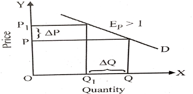
• Relatively Elastic Demand : Ep > 1

• Demand is relatively elastic when the percentage change in quantity demanded is greater than percentage change in price. In this case the demand curve is flatter as in Fig. And therefore ∆P < ∆Q.
• Examples : Most mid-range consumer durables like cars, T.V.s, air conditioner , commodities with several substitutes like unbranded garments.

These different degree of price elasticity.

1.8 INCOME ELASTICITY OF DEMAND

The measures the responsiveness of demand for a commodity to a commodity to a change in consumer’s income. The income elasticity of demand (Ey) is given by the percentage change in income, keeping constant all other variables, including price in the demand function .

Ey =

As with price elasticity, income elasticity can be found out by point or arc method. Point income elasticity of demand is given by

Ey = = •

Where, ∆Q = Change in quantity demanded

∆Y = Change in income

Q = Original quantity demanded

Y = Original income

1.9 CROSS ELASTICITY OF DEMAND

Price elasticity of demand for a commodity explains the changes in quantity demanded due to change in the price of the commodity. Demand for a commodity may change not only due to a change in its own price but due to the change in the price of  a substitute or complementary commodity. A change in demand for a commodity due to a change in the price of its substitute or complementary good is termed cross elasticity of demand. For example, if the price of Pepsi rises, Consumers may switch over to coke, assuming that there is no change in the price of coke .

Cross elasticity of demand (Ec) measures the responsiveness in the demand for commodity X to a change in the price of commodity Y. It is given by the percentage change in the quantity demanded for commodity X dividend by the percentage change in the price of commodity Y, keeping constant all other variables in the demand function. Thus,

Ec =

Questions:

1. What does law of demand explain?
2. What are the assumptions of law of demand?
3. What are the exceptions of law of demand?
4. What are the different types of elasticity?
5. State the different degrees of elasticity.
6. Suppose that the cross price elasticity of demand between bread and butter is – 0.5.What would you expect to happen to demand for butter if the price of bread rises by 10 percent?
7. A 10 percent increase in income brings about a 15 percent decreases in the demand for a good. What is the income elasticity of demand and is the normal good or an inferior good?