Unit 4

Production -Supply

4.1 Production

Production is a process of combining various material inputs and immaterial inputs (plans, know-how) in order to make something for consumption (output). It is the act of creating an output, a good or service which has value and contributes to the utility of individuals.

Supply

Supply is the number of goods and services that the suppliers are both willing and able to supply at a particular price during a given period of time. In this chapter, we will discuss more topics related to Supply.

Supply Schedule

The law of supply states that when the price of a commodity falls, its supply decreases and when the price of a commodity rises, its supply increases; other things remaining constant. Supply refers to the amount of quantity that a firm is willing to produce or offer for sale in the market. Supply schedule can be defined as a relation between the price of goods or services versus and the number of goods supplied. Now let us discuss the supply schedule in detail.

Supply Schedule

We can express the Supply of a commodity in the following three alternative ways:

1. Supply function
2. Supply schedule
3. Supply curve

Supply Function

The supply function of an individual supplier expresses his behaviour in relation to what he offers at the prevailing prices in the market in the algebraic form. In supply function, quantity supplied is expressed as a function of various variables.

SX = f(PX, CX, TX)

Where,

SX = Quantity supplied

PX = Price of the commodity

CX = Cost of production

TX = Technology of production

Supply Schedule

It is a statement in the form of a table that shows the different quantities of a commodity that a firm or a producer offers for sale in the market at different prices.

It denotes the relationship between the supply and the price, while all non-price variables remain constant. There are two types of Supply Schedules:

1. Individual Supply Schedule
2. Market Supply Schedule

Individual Supply Schedule

It is a supply schedule that depicts the supply by an individual firm or producer of a commodity in relation to its price. Let us understand it with the help of an example.

The above schedule depicts the individual supply schedule. We can see that when the price of the commodity is ₹100, its supply is 1000 units. Similarly, when its price is ₹500, its supply increases to 5000 units.

Thus, we can conclude that as the price falls the supply decreases and as the price rises the supply also increases. Hence, there exists a direct relationship between the price and quantity supplied.

Individual Supply Curve

It is a graphical representation of the individual supply schedule. The X-axis represents the supply and Y-axis represents the price of a commodity. There exists a direct relationship between price and quantity supplied of a commodity.

Market Supply Schedule

It is a summation of the individual supply schedules and depicts the supply of different customers for a commodity in relation to its price. Let us understand it with the help of an example.

The above schedule shows the market supply of commodity X. When the price of the commodity is ₹100, firm A supplies 1000 units while the firm B supplies 3000 units.

Thus, the market supply is 4000 units. Similarly, when its price is ₹500, firm A supplies 5000 units while firm B supplies 7000 units. Thus, it’s market demand increases to 12000 units.

Thus, we can conclude that whether it is the individual supply or the market supply, the law of supply governs both of them.

Market Supply Curve

It is a graphical representation of the market supply schedule. The X-axis represents the market supply in units and Y-axis represents the price of a commodity.

Production Function

Obviously, the factors of production (land, labor, capital, and entrepreneur) affect production, hence the name. However, this vague qualitative claim can’t tickle our economic bone. We need more quantifiable answers. And the production function serves the purpose. Let us take a look at the Cobb-Douglas Production Function.

Production Function

As discussed, the production function provides a quantitative perception of the relationship between the inputs and outputs. The inputs are the various factors of production- land, labour, capital, and enterprise whereas the outputs are the goods and services.

To put it differently, the production function can provide us with the maximum goods and services that we can produce using a given amount of inputs. Further, it can also help us in determining the inputs we require to achieve a minimum level of production. Note that a production function is defined for a given state of technology.

According to Richard H.Lefthich: The term production function is applicable to the physical relationship between a firm’s input of resources and its output of goods or services per unit of time leaving prices aside.

Moving away from complex definitions, we can say that the production function is a catalogue of output possibilities. Quantitatively, we can express the production function in the form of an equation in which the output is a dependent variable. Further, this output is a function of the inputs which are the independent variables. The equation is as follows:

q= f (a, b, c……, n)

Here ‘q’ stands for the rate of output of the given commodity and a, b, c, d…..n are the different inputs used per unit of time.

Cobb-Douglas Production Function

The Cobb-Douglas production function, named after Paul H. Douglas and C.W. Cobb, is a famous statistical production function. It was derived to study the whole of American manufacturing industries. The Cobb-Douglas production function is as follows:

Q= KLª[C^(l-a)]

Here Q is output, L is the quantity of labour, C is the quantity of capital, l and a are positive constants. This study led to the conclusion that labour contributes about 3/4th and capital about 1/4th of the increase in manufacturing production.

Short Run Vs. Long Run

Note that we can look at the production function through two-time frames- short run and long run. The short run is a short interval of time, in which we can change only the variable factors of production.

To point out, these variable factors are the ones which we can change over a small period of time, as the number of labour, raw material, fuel, power, etc. Symbolically, Q= T(K, L). Further, we do this with the help of the law of variable proportions.

On the other hand, the long run is a relatively much longer period of time. Obviously, in the long run, we can change all the factors of production i.e. both fixed and variable factors.

Hence, in the long run, we can change the factory size, techniques of production, machinery, to the number of labours, power, fuel and so on.

Thus the production function takes different forms according to the two-time frames. Evidently, we study production function with respect to two different time frames. The long-run production function is the subject matter of the law of returns to scale.

Assumptions of Production Function

The various assumptions of production function are:

1. It is related to a particular unit of time.
2. The technical knowledge during that time period remains constant.
3. The producer uses the best technique available.

Isoquant Curves

These lines represent various input combinations which produce the same levels of output. The producer can choose any of these combinations available to him because their outputs are always the same. Thus, we can also call them equal product curves or production indifference curves.

Just like indifference curves, isoquants are also negatively-sloping and convex in shape. They never intersect with each other. When there are more curves than one, the curve on the right represents greater output and curves on the left show less output.

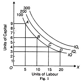
Consider the table below. It shows four combinations, i.e. A, B, C and D, which produce varying levels of output.

Plotting these figures on a graph provides us with this curve (Figure 1):

Source:Economicsdiscussion.net

The X-axis shows units of labour, while the Y-axis represents units of capital. Points A, B, C and D are combinations of factors on which IQ is the level of output, i.e. 100 units. IQ1 and IQ2 represent greater potential output.

Isocost Lines

Isocost lines represent combinations of two factors that can be bought with different outlays. In other words, it shows how we can spend money on two different factors to produce maximum output. These lines are also called budget lines or budget constraint lines.

Let’s assume that a farmer has Rs. 1,000 to spend on labour costs and ploughs for farming. The cost of one such plough and wage per labourer is Rs. 100. Considering his total outlay of Rs. 1,000, he can spend that money in the following combinations:

The farmer, in this case, can either spend the entire sum of Rs. 1,000 on just ploughs by buying 10 of them. Similarly, he can also spend it all on labour by employing 10 labourers. He can even purchase both, labour and ploughs using different combinations as shown above. The total outlay of Rs. 1,000 will remain the same. Hence, the isocost line will remain straight as shown below:

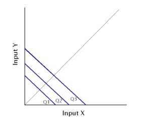
The x-axis represents units of ploughs, and Y-axis would show units of labour. Output levels are shown by a straight line because they remain constant.

Law of Variable Proportions or Returns to a Factor

This law exhibits the short-run production functions in which one factor varies while the others are fixed.

Also, when you obtain extra output on applying an extra unit of the input, then this output is either equal to or less than the output that you obtain from the previous unit.

The Law of Variable Proportions concerns itself with the way the output changes when you increase the number of units of a variable factor. Hence, it refers to the effect of the changing factor-ratio on the output.

In other words, the law exhibits the relationship between the units of a variable factor and the amount of output in the short-term. This is assuming that all other factors are constant. This relationship is also called returns to a variable factor.

The law states that keeping other factors constant, when you increase the variable factor, then the total product initially increases at an increases rate, then increases at a diminishing rate, and eventually starts declining.

Why is it called the Law of Variable Proportions?

As one input varies and all others remain constant, the factor ratio or the factor proportion varies. Let’s look at an example to understand this better:

Let’s say that you have 10 acres of land and 1 unit of labour . Therefore, the land-labour ratio is 10:1. Now, if you keep the land constant but increase the units of labour to 2, the land-labour ratio becomes 5:1.

Therefore, as you can see, the law analyses the effects of a change in the factor ratio on the amount of out and hence called the Law of Variable Proportions.

Law of Variable Proportions Explained

Let’s understand this law with the help of another example:

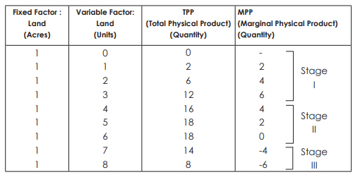
In this example, the land is the fixed factor and labour is the variable factor. The table shows the different amounts of output when you apply different units of labour to one acre of land which needs fixing.

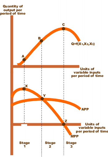
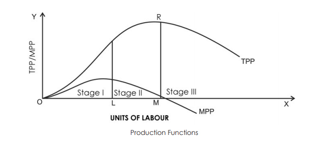
The following diagram explains the law of variable proportions. In order to make a simple presentation, we draw a Total Physical Product (TPP) curve and a Marginal Physical Product (MPP) curve as smooth curves against the variable input (labour).

Watch Videos on Law of Constant Proportion –

Three Stages of the Law

The law has three stages as explained below:

1. Stage I – The TPP increases at an increasing rate and the MPP increases too. The MPP increases with an increase in the units of the variable factor. Therefore, it is also called the stage of increasing returns. In this example, the Stage I of the law runs up to three units of labour (between the points O and L).
2. Stage II – The TPP continues to increase but at a diminishing rate. However, the increase is positive. Further, the MPP decreases with an increase in the no. of units of the variable factor. Hence, it is called the stage of diminishing returns. In this example, Stage II runs between four to six units of labour (between the points L and M). This stage reaches a point where TPP is maximum (18 in the above example) and MPP becomes zero (point R).
3. Stage III – Now, the TPP starts declining, MPP decreases and becomes negative. Therefore, it is called the stage of negative returns. In this example, Stage III runs between seven to eight units of labour (from the point M onwards).

Significance of the three stages

Stage I

A producer does not operate in Stage I. In this stage, the marginal product increases with an increase in the variable factor.

Therefore, the producer can employ more units of the variable to efficiently utilize the fixed factors. Hence, the producer would prefer to not stop in Stage I but will try to expand further.

Stage III

Producers do not like to operate in Stage III either. In this stage, there is a decline in total product and the marginal product becomes negative.

In order to increase the output, producers reduce the amount of variable factor. However, in Stage III, he incurs higher costs and also gets lesser revenue thereby getting reduced profits.

Stage II

Any rational producer avoids the first as well as third stages of production. Therefore, producers prefer Stage II – the stage of diminishing returns. This stage is the most relevant stage of operation for a producer according to the law of variable proportions.

Law of Variable Proportions in terms of TPP and MPP

The explanation is as follows:

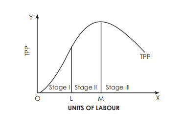
Law of Variable Proportions – in terms of TPP

We know that the law of variable proportions shows the relationship between units of a variable factor and the total physical product.

Also, if we keep other factors constant and increase the units of the variable factor, then the TPP initially increases at an increasing rate, then at a diminishing rate, and finally declines. Therefore, it has three clear stages:

1. I – TPP increasing at an increasing rate
2. II – TPP increasing at a diminishing rate
3. III – TPP declining

Example of Law of Variable Proportion in terms of TPP

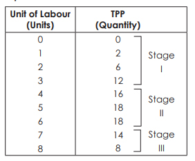
Diagram of Law of Variable Proportion in terms of TPP

Law of Variable Proportions in terms of MPP

The law also states that if we keep all other factors constant and increase the units of a variable factor, then the marginal physical product initially increases, then decreases, and finally becomes negative. Therefore, it has three stages:

1. I – MPP increasing
2. II – MPP decreasing but remaining positive
3. III – MPP continuing to decrease and becoming negative

Reason for the Operation of the Law

• In the short-term, we cannot vary all factors of production.
• In this case, there is only one variable factor while others are fixed.
• All other factors combine optimally to produce the maximum output.
• Before the point of optimum combination, if the units of a variable factor increase, then the factor proportion becomes more suitable and it leads to more efficient utilization of the fixed factors. Therefore, the marginal physical product increases.
• During the initial stages, the total product tends to rise at an increasing rate when the producer employs more units of a variable factor to the fixed factors.
• Subsequently, beyond the point of optimum combination, if the producer employs more units of the variable factor, then the factor proportion becomes inefficient. Therefore, the marginal product of that variable factor declines.
• Also, the producer sees a fall in the quantity of the fixed factor input per unit of the variable as he increases the units of the variable factor.
• Therefore, successive units of the variable input add decreasing amounts to the total output as they have less fixed inputs to work with.