Unit - 5

Curve Tracing

5.1 Tracing of Cartesian curves

Curve tracing - An introduction

A picture explains more clearly than words and numbers. A curve which is the image of functional relationship gives us a lot information about the relation. We can get information analyzing the equation itself but the associated curve is often easy and understandable.

Let’s study about how to trace the curves of various equations in different forms like Cartesian, parametric and polar.

Important definitions for curve tracing

Here are some terms that we use in curve tracing:

1. Double point- when a curve passes two times through this point is known as double point.

2. Node- a double point at which two real tangents can be drawn.(tangents should not be coincide)

3. Cusp -  a double point is a cusp when two tangents are coincide on it.

Asymptotes-

An asymptote of a curve of function y = f(x) is a line which does not intersect on the graph.

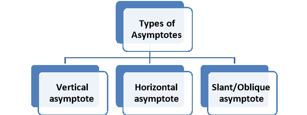
Types of asymptotes-

1. Vertical asymptote-

A line x = a which is straight is a vertical asymptote of the graph of the function y = f(x) if atleast one of the following condition does it follow-

Example: Determine the vertical asymptote of the function-

Sol. Here we have-

We can write the given function as-

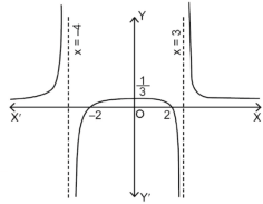
We can notice here as x gets closer to 3 from the left, then the value of the function gets smaller, approaching -∞ and x gets closer 3 from the right, then the value of the function gets larger and approaches +∞.

So that x = 3 is a vertical asymptote same as x = -4 is another vertical asymptote.

2. Horizontal asymptote-

A line y = L is called horizontal asymptote to the curve of the function f(x)-

If f(x)→ L as x→∞ or as x→-∞

Example: Find the horizontal asymptote of the function-

Sol. In order to find the horizontal asymptote-

=

Hence the horizontal asymptote is y = 2.

Example: Find the horizontal asymptote of the function-

Sol. Find the limits-

And

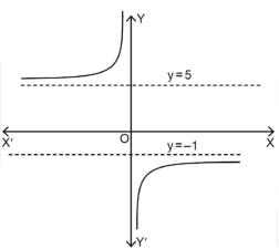
Hence the horizontal asymptotes are y = -1 and y = 5.

Figure will be as follows of the asymptotes of the given function-

3. Procedure to find the asymptotes parallel to axes of a polynomial function-

Theorem-

Suppose f(x , y) is a polynomial in x and y.

A straight line y = c is an asymptote of a curve f(x , y) = 0 if an only if y – c is a factor of the co-efficient of the highest power of x in f(x , y).

Example: Determine the asymptotes parallel to axes of the curve:

y² (x² - a²) = x

Sol. The given function can be written as-

y² (x² - a²) – x = 0

Asymptote parallel to x-axis-

Equating the coefficient of the highest power of x to zero, we get y² = 0 which means y = 0. This is an asymptote.

Asymptote parallel to y-axis-

Equating the coefficient of the highest power of x to zero, we get x² - a² = 0

Which gives x = ±a , that means x = +a , x = -a 

So that these are the asymptotes.

4. Oblique asymptote or slant asymptote-

A straight line y = mx + c where m ≠ 0 will be an oblique/slant asymptote to the graph of the function ‘f’ if-

Note- the value of m can be find as-

And the value of c can be find as-

c =

Example: Find the slant asymptotes of 

Sol. We have,

Which can be written as-

The value of ‘m’ will be-

=     = 

Now we can find ‘c’ as –

c = = =

= 0

Hence the slant asymptotes are

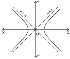
Example: Find the slant asymptote of the function f(x) = x + .

Sol. Find the value of m-

Hence the y = x + c,

Now find c-

Here c must not be infinite.

So we can say that f does not have a slant asymptote at ∞.

Tracing a curve- Cartesian form

Let us the equation of a curve is f(x,y)=0 , now we will learn few steps to simplify tracing of this curve.

1. The first step to find out the region of the plane. For example no point in the curve x= y² in second and third quadrant as we will always get a positive value on x-axis. That means our curve will lie on first and fourth quadrant only.

2. The second step is to find out If the curve is symmetrical about any line or origin.

Some examples of symmetrical curves are as below-

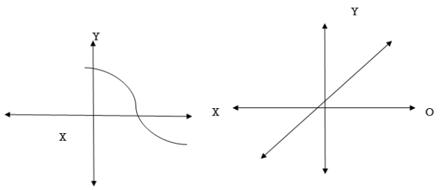
Symmetric about the x-axis                                             Symmetric about origin

Steps to determine the symmetry of a curve:

1. If all the powers of x in function f(x,y)=0 are even, then f(x,y)= f(-x,y) and the curve is always symmetrical about y-axis. Similarly we can draw the conclusion about x-axis

2.If f(x,y)= 0 & f(-x,-y)= 0 , then the curve is symmetrical about the origin.

3. If the equation of the curve does not change when we interchange x and y then it is symmetrical about the line y= x

Let’s understand this with the help of following table-

4. The next step to determine the points where curve intersects the axes. If we put y = 0 in f(x,y)=0 and solve the equation, we get the points interecting on x-axis. Smilarly we get point on y- axis.

5. Now we try to locate the points for discontinuity of the function.

6. Calculate dy/dx to locate the portion where the curve is rising(dy/dx>0) or falling(dy/dx<0)

7. Calculate d²y/dx² to locate maxima and minima and the point of inflection

For maxima = dy/dx = 0,  d²y/dx²<0      &     for minima = dy/dx = 0,  d²y/dx²>0

For point of inflection -  d²y/dx² = 0

8. The next step is to find the asymptotes,

9. Another point to determine the singular point. The shape of the curve at these points generally more complex.

10. Finally plot the points as many as we can. Also try to draw tangents to the curve at some points(calculate the derivative). Now join the plotted point by a smooth curve.

Now we will understand curve tracing with some easy examples:

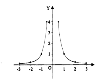
Example-:  Trace the curve y = 1/x².

Sol.         

As we can see y- coordinates of the curve can not be negative. So the                                              curve must be above x-axis. The curve is also symmetric about y-axis so we can draw the graph only in single side.

Here, we will find the first and second derivatives-

So, dy/dx= -2/x³ and d²y/dx² = 6/ x⁴    ,  here  dy/dx <0 for all x>0 so we can say that the function is non- increasing so the graph falls as we increase x.

Also second derivative is also non zero so there are no point of inflection.

Here the curve is x²y=1 (rewritten), here both the axes are asymptotes of the curve.

Here is the figure of the curve-:

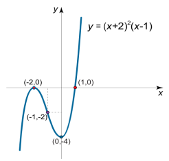
Example-2: Trace the curve y= (x+2)²(x-1).

Sol. Here first we check the slant asymptotes (there is no vertical asymptote)

So, p =

=

=

=

=  ) = +

Since p is infinity then the function has no slant asymptotes.

Now we will find the point of intersection with axes:

Y(0)= -4;

Put y(x)= 0,     (x+2)²(x-1)= 0

We get by solving,       X1= -2,     x2= 1

Now calculate the first derivative,

Here we will find stationary point by putting first derivative equal to zero:

3x(x+2) = 0

X1 = 0,   x2 = -2

X= -2 is maximum and x= 0 is minimum point.

The value of the function at these points will be:

Y= -4, 0

Now we will find second derivative:

Now, d²y/dx² = 6x+6,

So the function is strictly upward for:

X<-1,

And strictly downward for

x>-1,

Hence x= -1 is the inflection point

We get    y(-1)= -2

Here is the figure of curve:

5.2 Tracing of polar curves

Tracing a curve- polar form

To trace the polar curve r = f ( we follow the following steps:

1. Symmetry – (a) if the equation is an even function of , then the curve is symmetrical about the initial line.

(b) if the equation is an even function of r, then the curve is symmetrical about the origin/

(C ). If the equation remains same if we change by - and r by –r then the curve is symmetric about the line through the pole and perpendicular to the initial line.

2. Region- Find the reason for for which r is defined and real

3. Table- make table for the values of r determined by .

4. Angle -  is the angle between the radius vector and tangent to the curve;

= )

Then angle = +, tangents to the curve can be determined by angle

5. Asymptotes-   find the asymptotes of the curve.

Now we will understand of tracing of polar equations by an example:

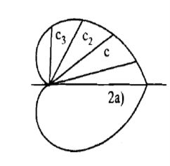
Example: Trace the curve r = a(1+ cos.

Sol.    Here we can see clearly cos = cos(-), hence the curve is symmetric about initial line.

Since -1, the curve lies inside the circle r = 2a

= -asin , when  0, thus r decreases as increases in the interval 0 to

	0
r	2a	A	0

= - cot () = tan(+ ),      this shows the angle between r and and the tangent is 0 or according to   0 or . Hence the line joining a point on the curve to the origin is orthogonal to the tangent when = 0 and coincides with

From the above results, we can easily draw the graph above the initial line

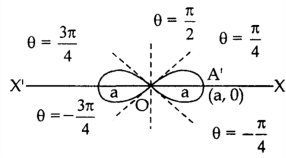
Example-2:  Trace the curve  .

Sol. Symmetry about initial line- Put r = 0,

Hence the straight line are the tangents to the curve at the pole.

Values of ‘r’ as changes from 0 to π-

Table for the values of ‘r’-

	0	0
		Imaginary
	0	0

Here according to the table the curve does not exist for the value lying between 
to

The figure will be as follows of the curve-

Key takeaways-

1. An asymptote of a curve of function y = f(x) is a line which does not intersect on the graph.

2. Double point- when a curve passes two times through this point is known as double point.

3. Node- a double point at which two real tangents can be drawn.(tangents should not be coincide)

4. Cusp -  a double point is a cusp when two tangents are coincide on it.

5.3 Tracing of parametric curves

Tracing a curve- parametric form

Before we start tracing curves of the equations in parametric form, here first we understand the definition of parametric equations:

Parametric equations:

If x and y are the continuous functions of “t” on an interval I , then the equations:

x = x(t)

And

y= y(t)

Are called parametric equations and t is called the parameter.

Now let’s understand how to trace the curves in parametric by examples:

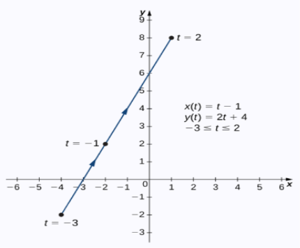
Example1: trace the curve of the following parametric equations:

x(t) = t-1 ,     y(t) = 2t+4         -3<

Sol.  Here we will create the table for t, x(t) and y(t) , t is independent variable in both case,

Here value of t lies between -3 to 2.

By plotting these set of point we get a curve as below.

Arrows in the graph indicates the orientation of the graph.

References:

1. E. Kreyszig, “Advanced Engineering Mathematics”, John Wiley & Sons, 2006.
2. P. G. Hoel, S. C. Port And C. J. Stone, “Introduction To Probability Theory”, Universal Book Stall, 2003.
3. S. Ross, “A First Course in Probability”, Pearson Education India, 2002.
4. W. Feller, “An Introduction To Probability Theory and Its Applications”, Vol. 1, Wiley, 1968.
5. N.P. Bali and M. Goyal, “A Text Book of Engineering Mathematics”, Laxmi Publications, 2010.
6. B.S. Grewal, “Higher Engineering Mathematics”, Khanna Publishers, 2000.