Unit - 2
Solution of linear simultaneous Equations
In this method we eliminate successively the unknown  so that the equation (1) remain with the single unknown
  and reduce to upper triangular system. At last with help of back substitution we calculate the values of the remaining unknowns.
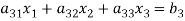
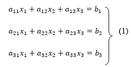
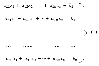
Consider a system of n linear equation in n unknown 

To convert the above system into upper triangular matrix we eliminate  from the second, third, fourth …., n equations above by multiplying the first equation by
 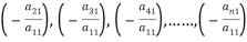 added them to the corresponding equations second, third, fourth,…., n equation. We get

… …… ….. …
… …… …. …

Repeating the above method for  we get finally the upper triangular form.
Upper Triangular form of above

Thus  .
.
Then we calculate the values of  .
.
Note: In (i) the coefficient  is the pivot element and the equation is called the pivot equation. If
  then the above method fails and if it is close to zero the round off error may occur.
If  or very small compared to other coefficient of the equation, then we find the largest available coefficient in the column given below the pivot equation and then interchange the two rows to obtain new pivot variable this is known as partial pivoting.
Example 1
Apply Gauss Elimination method to solve the equations:

Given Check Sum (sum of coefficient and constant)
 -1 …. (I)
 -16 …. (ii)
 5…. (iii)
(I)We eliminate x from (ii) and (iii)
Apply eq(ii)-eq(i) and eq(iii)-3eq(i) we get
 -1 ….(i)
 -15 ….(iv)
 8 ….(v)
(II) We eliminate y from eq(v)
Apply 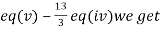
 -1 ….(i)
 -15 ….(iv)
 73 ….(vi)
(III) Back Substitution we get
From (vi) we get 
From (iv) we get 
From (i) we get 
Hence the solution of the given equation is 
Example 2:
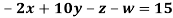
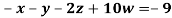
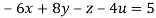
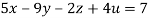
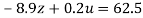
Solve the equation by Gauss Elimination Method:

Given 

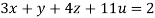

Rewrite the given equation as
 … (i)
… (i)
 ….(ii)
 ….(iii)
 …(iv)
…(iv)
(I) We eliminate x from (ii),(iii) and (iv) we get
Apply eq(ii) + 6eq(i), eq(iii) -3eq(i), eq(iv)-5eq(i) we get
 …(i)
…(i)
 ….(v)
….(v)
 ….(vi)
 …(vii)
(II) We eliminate y from (vi) and (vii) we get
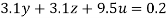
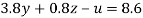
Apply 3.8 eq(vi)-3.1eq(v) and 3.8eq(vii)+5.5eq(v) we get
 …(i)
…(i)
 ….(v)
….(v)
 …(viii)
 …(ix)
…(ix)
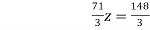
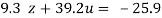
(III) We eliminate z from eq (ix) we get
Apply 9.3eq (ix) + 8.3eq (viii), we get
 … (i)
… (i)
 ….(v)
….(v)
 …(viii)
350.74u=350.74
Or u = 1
(IV) Back Substitution
From eq(viii) 
Form eq(v), we get 
From eq(i) , 
Hence the solution of the given equation is x=5, y=4, z=-7 and u=1.
Example 3:
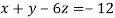
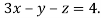
Apply Gauss Elimination Method to solve the following system of equation:

Given  … (i)
… (i)
 … (ii)
 … (iii)
(I) We eliminate x from (ii) and (iii)
Apply  we get
 … (i)
… (i)
 … (iv)
 … (v)
… (v)
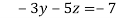
(II) We eliminate y from (v)
Apply we get
 … (i)
… (i)
 … (vi)
 … (vii)
(III) Back substitution
From (vii) 
From (vi) 
From (i) 
Hence the solution of the equation is 
Example 4: Solve the system by Gauss Elimination method using partial pivoting


Given exact solution is 
Given equations are 

Using partial pivoting we rewrite the given equations as
 (1)
(1)
 (2)
(2)
Using Gauss elimination method
Multiplying (1) by (-0.0003120/0.5000) + (2) we get

Or 
Substituting value of y in equation (1) we get 
Hence 
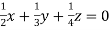
Example 5: Solve the system of linear equations


Using partial pivoting by Gauss elimination method we rewrite the given equations as
 (1)
(1)
 (2)
(2)
 (3)
(3)
Apply 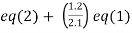 and
and 
 (1)
(1)
 (4)
(4)
 (5)
(5)
Apply  )
)
 (1)
(1)
 (4)
(4)

Or  .
.
Putting value of z in  we get
  .
.
Putting values of y and z in  we get
  .
.
Hence the solution of the equation is  .
.
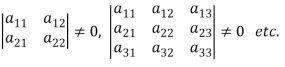
The method is based on the fact that every matrix A can be expressed as the product of a lower triangular matrix and an upper triangular matrix , provided all the principal minors of A are non-singular.
Which means-
If  , then-

Now consider the equations-


We can write it as-

Where-
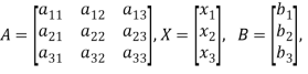
Let

Where-

Equation (1) becomes-

Writing-

Equation (3) becomes-
 which is equivalent to the equations-

Solving these for  we know V. Then equation (4) becomes-

From which  can be found by back substitution.
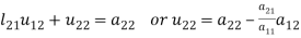
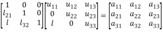
We write (2) as to find the matrix L and U-

Multiplying the matrix on the left and equating corresponding elements from both sides, we get-


3. 

4. 
5. 
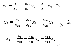
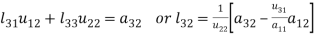
We compute the elements of L and U in the following manner-
- First row of U
- First column of L
- Second row of U
- Second column of L
- Third row of U
Example: Solve the equations-


Sol.
Let

So that-


3. 

4. 
5. 
So

Thus-
Writing UX = V,
The system of given equations become-

By solving this-
We get-


Therefore the given system becomes-

Which means-

By back substitution, we get the values of x, y and z.
Jacobi’s Iteration method and Gauss-Seidal method:
Let us consider the system of simultaneous linear equation
The coefficients of the diagonal elements are larger than the all other coefficients and are non zero. Rewrite the above equation we get

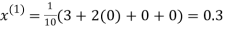
Take the initial approximation  we get the values of the first approximation of
 .
.
By the successive iteration we will get the desired the result.
Example 1 Use Jacobi’s method to solve the system of equations:

Since 
So, we express the unknown with large coefficient in terms of other coefficients.

Let the initial approximation be 


 2.35606
 0.91666


 1.932936
 0.831912

 3.016873
 1.969654


 3.010217
 1.986010


 1.988631
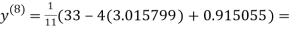
 0.915055


 1.986532
 0.911609


 1.985792
 0.911547


 1.98576
 0.911698
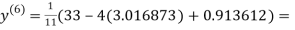
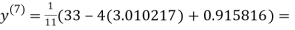
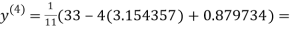
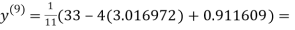
Since the approximation in ninth and tenth iteration is same up to three decimal places, hence the solution of the given equations is 
Example 2 Solve by Jacobi’s Method, the equations

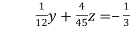
Given equation can be rewrite in the form
 … (i)
… (i)
 ..(ii)
 ..(iii)
Let the initial approximation be 

Putting these values on the right of the equation (i), (ii) and (iii) and so we get


Putting these values on the right of the equation (i), (ii) and (iii) and so we get


Putting these values on the right of the equation (i), (ii) and (iii) and so we get
 0.90025


Putting these values on the right of the equation (i), (ii) and (iii) and so we get


Putting these values on the right of the equation (i), (ii) and (iii) and so we get


Hence solution approximately is 
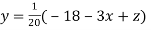
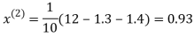
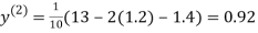
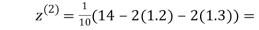
Example 3 Use Jacobi’s method to solve the system of the equations

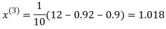
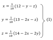
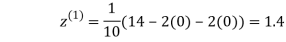
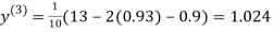
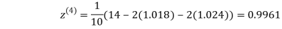
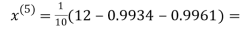
Rewrite the given equations

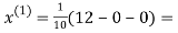
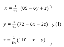
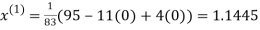
Let the initial approximation be 

 1.2
1.2
 1.3
1.3


 0.9
0.9


 1.03
1.03

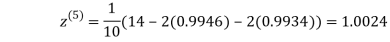
 0.9946
 0.9934


 1.0015


Hence the solution of the above equation correct to two decimal places is
Gauss Seidel method:
This is the modification of the Jacobi’s Iteration. As above in Jacobi’s Iteration, we take first approximation as  and put in the right hand side of the first equation of (2) and let the result be
  . Now we put
  right hand side of second equation of (2) and suppose the result is
  now put
  in the RHS of third equation of (2) and suppose the result be
  the above method is repeated till the values of all the unknown are found up to desired accuracy.
Example 1 Use Gauss –Seidel Iteration method to solve the system of equations

Since 
So, we express the unknown of larger coefficient in terms of the unknowns with smaller coefficients.
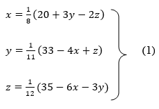
Rewrite the above system of equations

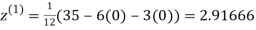
Let the initial approximation be 

 3.14814
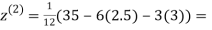


 2.43217


 2.42571


 2.4260


Hence the solution correct to three decimal places is

Example 2 Solve the following system of equations
 By Gauss-Seidel method.
Rewrite the given system of equations as

Let the initial approximation be 


Thus the required solution is 
Example 3 Solve the following equations by Gauss-Seidel Method


Rewrite the above system of equations

Let the initial approximation be 


Hence the required solution is 
References:
- E. Kreyszig, “Advanced Engineering Mathematics”, John Wiley & Sons, 2006.
- P. G. Hoel, S. C. Port And C. J. Stone, “Introduction To Probability Theory”, Universal Book Stall, 2003.
- S. Ross, “A First Course in Probability”, Pearson Education India, 2002.
- W. Feller, “An Introduction To Probability Theory and Its Applications”, Vol. 1, Wiley, 1968.
- N.P. Bali and M. Goyal, “A Text Book of Engineering Mathematics”, Laxmi Publications, 2010.
- B.S. Grewal, “Higher Engineering Mathematics”, Khanna Publishers, 2000.
Unit - 2
Solution of linear simultaneous Equations
In this method we eliminate successively the unknown  so that the equation (1) remain with the single unknown
  and reduce to upper triangular system. At last with help of back substitution we calculate the values of the remaining unknowns.
Consider a system of n linear equation in n unknown 

To convert the above system into upper triangular matrix we eliminate  from the second, third, fourth …., n equations above by multiplying the first equation by
  added them to the corresponding equations second, third, fourth,…., n equation. We get


… …… ….. …
… …… …. …

Repeating the above method for  we get finally the upper triangular form.
Upper Triangular form of above

Thus  .
.
Then we calculate the values of  .
.
Note: In (i) the coefficient  is the pivot element and the equation is called the pivot equation. If
  then the above method fails and if it is close to zero the round off error may occur.
If  or very small compared to other coefficient of the equation, then we find the largest available coefficient in the column given below the pivot equation and then interchange the two rows to obtain new pivot variable this is known as partial pivoting.
Example 1
Apply Gauss Elimination method to solve the equations:

Given Check Sum (sum of coefficient and constant)
 -1 …. (I)
 -16 …. (ii)
 5…. (iii)
(I)We eliminate x from (ii) and (iii)
Apply eq(ii)-eq(i) and eq(iii)-3eq(i) we get
 -1 ….(i)
 -15 ….(iv)
 8 ….(v)
(II) We eliminate y from eq(v)
Apply 
 -1 ….(i)
 -15 ….(iv)
 73 ….(vi)
(III) Back Substitution we get
From (vi) we get 
From (iv) we get 
From (i) we get 
Hence the solution of the given equation is 
Example 2:
Solve the equation by Gauss Elimination Method:

Given 


Rewrite the given equation as
 … (i)
… (i)
 ….(ii)
 ….(iii)
 …(iv)
…(iv)
(I) We eliminate x from (ii),(iii) and (iv) we get
Apply eq(ii) + 6eq(i), eq(iii) -3eq(i), eq(iv)-5eq(i) we get
 …(i)
…(i)
 ….(v)
….(v)
 ….(vi)
 …(vii)
(II) We eliminate y from (vi) and (vii) we get
Apply 3.8 eq(vi)-3.1eq(v) and 3.8eq(vii)+5.5eq(v) we get
 …(i)
…(i)
 ….(v)
….(v)
 …(viii)
 …(ix)
…(ix)
(III) We eliminate z from eq (ix) we get
Apply 9.3eq (ix) + 8.3eq (viii), we get
 … (i)
… (i)
 ….(v)
….(v)
 …(viii)
350.74u=350.74
Or u = 1
(IV) Back Substitution
From eq(viii) 
Form eq(v), we get 
From eq(i) , 
Hence the solution of the given equation is x=5, y=4, z=-7 and u=1.
Example 3:
Apply Gauss Elimination Method to solve the following system of equation:

Given  … (i)
… (i)
 … (ii)
 … (iii)
(I) We eliminate x from (ii) and (iii)
Apply  we get
 … (i)
… (i)
 … (iv)
 … (v)
… (v)
(II) We eliminate y from (v)
Apply we get
 … (i)
… (i)
 … (vi)
 … (vii)
(III) Back substitution
From (vii) 
From (vi) 
From (i) 
Hence the solution of the equation is 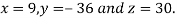
Example 4: Solve the system by Gauss Elimination method using partial pivoting


Given exact solution is 
Given equations are 

Using partial pivoting we rewrite the given equations as
 (1)
(1)
 (2)
(2)
Using Gauss elimination method
Multiplying (1) by (-0.0003120/0.5000) + (2) we get

Or 
Substituting value of y in equation (1) we get 
Hence 
Example 5: Solve the system of linear equations


Using partial pivoting by Gauss elimination method we rewrite the given equations as
 (1)
(1)
 (2)
(2)
 (3)
(3)
Apply  and
and 
 (1)
(1)
 (4)
(4)
 (5)
(5)
Apply  )
)
 (1)
(1)
 (4)
(4)

Or  .
.
Putting value of z in  we get
  .
.
Putting values of y and z in  we get
  .
.
Hence the solution of the equation is  .
.
The method is based on the fact that every matrix A can be expressed as the product of a lower triangular matrix and an upper triangular matrix , provided all the principal minors of A are non-singular.
Which means-
If  , then-


Now consider the equations-


We can write it as-

Where-

Let

Where-

Equation (1) becomes-

Writing-

Equation (3) becomes-
 which is equivalent to the equations-

Solving these for  we know V. Then equation (4) becomes-

From which  can be found by back substitution.
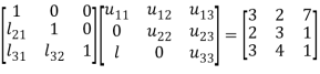
We write (2) as to find the matrix L and U-

Multiplying the matrix on the left and equating corresponding elements from both sides, we get-


3. 

4. 
5. 
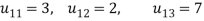
We compute the elements of L and U in the following manner-
- First row of U
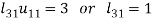
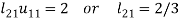
- First column of L
- Second row of U
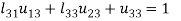
- Second column of L
- Third row of U
Example: Solve the equations-


Sol.
Let
So that-

3. 

4. 
5. 
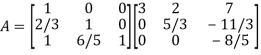
So

Thus-

Writing UX = V,
The system of given equations become-
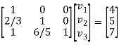
By solving this-
We get-


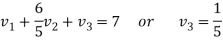
Therefore the given system becomes-

Which means-

By back substitution, we get the values of x, y and z.
Jacobi’s Iteration method and Gauss-Seidal method:
Let us consider the system of simultaneous linear equation

The coefficients of the diagonal elements are larger than the all other coefficients and are non zero. Rewrite the above equation we get
Take the initial approximation 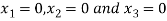 we get the values of the first approximation of
 .
.
By the successive iteration we will get the desired the result.
Example 1 Use Jacobi’s method to solve the system of equations:

Since 
So, we express the unknown with large coefficient in terms of other coefficients.
Let the initial approximation be 


 2.35606
 0.91666


 1.932936
 0.831912

 3.016873
 1.969654


 3.010217
 1.986010


 1.988631
 0.915055


 1.986532
 0.911609


 1.985792
 0.911547


 1.98576
 0.911698
Since the approximation in ninth and tenth iteration is same up to three decimal places, hence the solution of the given equations is 
Example 2 Solve by Jacobi’s Method, the equations

Given equation can be rewrite in the form
 … (i)
… (i)
 ..(ii)
 ..(iii)
Let the initial approximation be 

Putting these values on the right of the equation (i), (ii) and (iii) and so we get


Putting these values on the right of the equation (i), (ii) and (iii) and so we get


Putting these values on the right of the equation (i), (ii) and (iii) and so we get
 0.90025


Putting these values on the right of the equation (i), (ii) and (iii) and so we get


Putting these values on the right of the equation (i), (ii) and (iii) and so we get


Hence solution approximately is 
Example 3 Use Jacobi’s method to solve the system of the equations

Rewrite the given equations

Let the initial approximation be 

 1.2
1.2
 1.3
1.3


 0.9
0.9


 1.03
1.03

 0.9946
 0.9934


 1.0015


Hence the solution of the above equation correct to two decimal places is

Gauss Seidel method:
This is the modification of the Jacobi’s Iteration. As above in Jacobi’s Iteration, we take first approximation as  and put in the right hand side of the first equation of (2) and let the result be
  . Now we put
  right hand side of second equation of (2) and suppose the result is
  now put
  in the RHS of third equation of (2) and suppose the result be
  the above method is repeated till the values of all the unknown are found up to desired accuracy.
Example 1 Use Gauss –Seidel Iteration method to solve the system of equations

Since 
So, we express the unknown of larger coefficient in terms of the unknowns with smaller coefficients.
Rewrite the above system of equations

Let the initial approximation be 

 3.14814


 2.43217


 2.42571


 2.4260


Hence the solution correct to three decimal places is

Example 2 Solve the following system of equations
 By Gauss-Seidel method.
Rewrite the given system of equations as

Let the initial approximation be 


Thus the required solution is 
Example 3 Solve the following equations by Gauss-Seidel Method


Rewrite the above system of equations

Let the initial approximation be 


Hence the required solution is 
References:
- E. Kreyszig, “Advanced Engineering Mathematics”, John Wiley & Sons, 2006.
- P. G. Hoel, S. C. Port And C. J. Stone, “Introduction To Probability Theory”, Universal Book Stall, 2003.
- S. Ross, “A First Course in Probability”, Pearson Education India, 2002.
- W. Feller, “An Introduction To Probability Theory and Its Applications”, Vol. 1, Wiley, 1968.
- N.P. Bali and M. Goyal, “A Text Book of Engineering Mathematics”, Laxmi Publications, 2010.
- B.S. Grewal, “Higher Engineering Mathematics”, Khanna Publishers, 2000.
Unit - 2
Solution of linear simultaneous Equations
Unit - 2
Solution of linear simultaneous Equations
Unit - 2
Solution of linear simultaneous Equations
Unit - 2
Solution of linear simultaneous Equations
Unit - 2
Solution of linear simultaneous Equations
In this method we eliminate successively the unknown  so that the equation (1) remain with the single unknown
  and reduce to upper triangular system. At last with help of back substitution we calculate the values of the remaining unknowns.
Consider a system of n linear equation in n unknown 
To convert the above system into upper triangular matrix we eliminate  from the second, third, fourth …., n equations above by multiplying the first equation by
  added them to the corresponding equations second, third, fourth,…., n equation. We get


… …… ….. …
… …… …. …

Repeating the above method for  we get finally the upper triangular form.
Upper Triangular form of above

Thus  .
.
Then we calculate the values of  .
.
Note: In (i) the coefficient  is the pivot element and the equation is called the pivot equation. If
  then the above method fails and if it is close to zero the round off error may occur.
If  or very small compared to other coefficient of the equation, then we find the largest available coefficient in the column given below the pivot equation and then interchange the two rows to obtain new pivot variable this is known as partial pivoting.
Example 1
Apply Gauss Elimination method to solve the equations:

Given Check Sum (sum of coefficient and constant)
 -1 …. (I)
 -16 …. (ii)
 5…. (iii)
(I)We eliminate x from (ii) and (iii)
Apply eq(ii)-eq(i) and eq(iii)-3eq(i) we get
 -1 ….(i)
 -15 ….(iv)
 8 ….(v)
(II) We eliminate y from eq(v)
Apply 
 -1 ….(i)
 -15 ….(iv)
 73 ….(vi)
(III) Back Substitution we get
From (vi) we get 
From (iv) we get 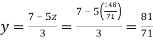
From (i) we get 
Hence the solution of the given equation is 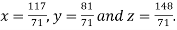
Example 2:
Solve the equation by Gauss Elimination Method:

Given 


Rewrite the given equation as
 … (i)
… (i)
 ….(ii)
 ….(iii)
 …(iv)
…(iv)
(I) We eliminate x from (ii),(iii) and (iv) we get
Apply eq(ii) + 6eq(i), eq(iii) -3eq(i), eq(iv)-5eq(i) we get
 …(i)
…(i)
 ….(v)
….(v)
 ….(vi)
 …(vii)
(II) We eliminate y from (vi) and (vii) we get
Apply 3.8 eq(vi)-3.1eq(v) and 3.8eq(vii)+5.5eq(v) we get
 …(i)
…(i)
 ….(v)
….(v)
 …(viii)
 …(ix)
…(ix)
(III) We eliminate z from eq (ix) we get
Apply 9.3eq (ix) + 8.3eq (viii), we get
 … (i)
… (i)
 ….(v)
….(v)
 …(viii)
350.74u=350.74
Or u = 1
(IV) Back Substitution
From eq(viii) 
Form eq(v), we get 
From eq(i) , 
Hence the solution of the given equation is x=5, y=4, z=-7 and u=1.
Example 3:
Apply Gauss Elimination Method to solve the following system of equation:

Given 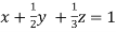 … (i)
… (i)
 … (ii)
 … (iii)
(I) We eliminate x from (ii) and (iii)
Apply  we get
 … (i)
… (i)
 … (iv)
 … (v)
… (v)
(II) We eliminate y from (v)
Apply we get
 … (i)
… (i)
 … (vi)
 … (vii)
(III) Back substitution
From (vii) 
From (vi) 
From (i) 
Hence the solution of the equation is 
Example 4: Solve the system by Gauss Elimination method using partial pivoting


Given exact solution is 
Given equations are 

Using partial pivoting we rewrite the given equations as
 (1)
(1)
 (2)
(2)
Using Gauss elimination method
Multiplying (1) by (-0.0003120/0.5000) + (2) we get

Or 
Substituting value of y in equation (1) we get 
Hence 
Example 5: Solve the system of linear equations


Using partial pivoting by Gauss elimination method we rewrite the given equations as
 (1)
(1)
 (2)
(2)
 (3)
(3)
Apply  and
and 
 (1)
(1)
 (4)
(4)
 (5)
(5)
Apply  )
)
 (1)
(1)
 (4)
(4)
Or  .
.
Putting value of z in  we get
  .
.
Putting values of y and z in  we get
  .
.
Hence the solution of the equation is  .
.
The method is based on the fact that every matrix A can be expressed as the product of a lower triangular matrix and an upper triangular matrix , provided all the principal minors of A are non-singular.
Which means-
If  , then-


Now consider the equations-


We can write it as-

Where-

Let

Where-

Equation (1) becomes-

Writing-

Equation (3) becomes-
 which is equivalent to the equations-

Solving these for  we know V. Then equation (4) becomes-

From which  can be found by back substitution.
We write (2) as to find the matrix L and U-
Multiplying the matrix on the left and equating corresponding elements from both sides, we get-


3. 

4. 
5. 
We compute the elements of L and U in the following manner-
- First row of U
- First column of L
- Second row of U
- Second column of L
- Third row of U
Example: Solve the equations-


Sol.
Let

So that-


3. 

4. 
5. 
So

Thus-

Writing UX = V,
The system of given equations become-

By solving this-
We get-


Therefore the given system becomes-
Which means-

By back substitution, we get the values of x, y and z.
Jacobi’s Iteration method and Gauss-Seidal method:
Let us consider the system of simultaneous linear equation

The coefficients of the diagonal elements are larger than the all other coefficients and are non zero. Rewrite the above equation we get

Take the initial approximation  we get the values of the first approximation of
 .
.
By the successive iteration we will get the desired the result.
Example 1 Use Jacobi’s method to solve the system of equations:

Since 
So, we express the unknown with large coefficient in terms of other coefficients.

Let the initial approximation be 


 2.35606
 0.91666


 1.932936
 0.831912

 3.016873
 1.969654


 3.010217
 1.986010


 1.988631
 0.915055


 1.986532
 0.911609


 1.985792
 0.911547


 1.98576
 0.911698
Since the approximation in ninth and tenth iteration is same up to three decimal places, hence the solution of the given equations is 
Example 2 Solve by Jacobi’s Method, the equations

Given equation can be rewrite in the form
 … (i)
… (i)
 ..(ii)
 ..(iii)
Let the initial approximation be 

Putting these values on the right of the equation (i), (ii) and (iii) and so we get


Putting these values on the right of the equation (i), (ii) and (iii) and so we get


Putting these values on the right of the equation (i), (ii) and (iii) and so we get
 0.90025


Putting these values on the right of the equation (i), (ii) and (iii) and so we get


Putting these values on the right of the equation (i), (ii) and (iii) and so we get


Hence solution approximately is 
Example 3 Use Jacobi’s method to solve the system of the equations

Rewrite the given equations
Let the initial approximation be 

 1.2
1.2
 1.3
1.3


 0.9
0.9


 1.03
1.03

 0.9946
 0.9934

 1.0015

Hence the solution of the above equation correct to two decimal places is

Gauss Seidel method:
This is the modification of the Jacobi’s Iteration. As above in Jacobi’s Iteration, we take first approximation as  and put in the right hand side of the first equation of (2) and let the result be
  . Now we put
 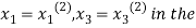 right hand side of second equation of (2) and suppose the result is
  now put
  in the RHS of third equation of (2) and suppose the result be
  the above method is repeated till the values of all the unknown are found up to desired accuracy.
Example 1 Use Gauss –Seidel Iteration method to solve the system of equations

Since 
So, we express the unknown of larger coefficient in terms of the unknowns with smaller coefficients.
Rewrite the above system of equations
Let the initial approximation be 

 3.14814


 2.43217


 2.42571


 2.4260


Hence the solution correct to three decimal places is

Example 2 Solve the following system of equations
 By Gauss-Seidel method.
Rewrite the given system of equations as

Let the initial approximation be 


Thus the required solution is 
Example 3 Solve the following equations by Gauss-Seidel Method


Rewrite the above system of equations

Let the initial approximation be 


Hence the required solution is 
References:
- E. Kreyszig, “Advanced Engineering Mathematics”, John Wiley & Sons, 2006.
- P. G. Hoel, S. C. Port And C. J. Stone, “Introduction To Probability Theory”, Universal Book Stall, 2003.
- S. Ross, “A First Course in Probability”, Pearson Education India, 2002.
- W. Feller, “An Introduction To Probability Theory and Its Applications”, Vol. 1, Wiley, 1968.
- N.P. Bali and M. Goyal, “A Text Book of Engineering Mathematics”, Laxmi Publications, 2010.
- B.S. Grewal, “Higher Engineering Mathematics”, Khanna Publishers, 2000.


