Unit - 5
Linear Equations and Matrix Theory
Introduction:
Matrices has wide range of applications in various disciplines such as chemistry, Biology, Engineering, Statistics, economics, etc.
Matrices play an important role in computer science also.
Matrices are widely used to solving the system of linear equations, system of linear differential equations and non-linear differential equations.
First time the matrices were introduced by Cayley in 1860.
Definition-
A matrix is a rectangular arrangement of the numbers.
These numbers inside the matrix are known as elements of the matrix.
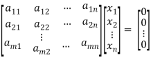
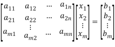
A matrix ‘A’ is expressed as-
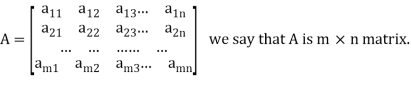
The vertical elements are called columns and the horizontal elements are rows of the matrix.
The order of matrix A is m by n or (m× n)
Notation of a matrix-
A matrix ‘A’ is denoted as-
A = 
Where, i = 1, 2, …….,m and j = 1,2,3,…….n
Here ‘i’ denotes row and ‘j’ denotes column.
Types of matrices-
1. Rectangular matrix-
A matrix in which the number of rows is not equal to the number of columns, are called rectangular matrix.
Example:
A = 
The order of matrix A is 2×3 , that means it has two rows and three columns.
Matrix A is a rectangular matrix.
2. Square matrix-
A matrix which has equal number of rows and columns, is called square matrix.
Example:
A = 
The order of matrix A is 3 ×3 , that means it has three rows and three columns.
Matrix A is a square matrix.
3. Row matrix-
A matrix with a single row and any number of columns is called row matrix.
Example:
A = 
4. Column matrix-
A matrix with a single column and any number of rows is called row matrix.
Example:
A = 
5. Null matrix (Zero matrix)-
A matrix in which each element is zero, then it is called null matrix or zero matrix and denoted by O
Example:
A = 
6. Diagonal matrix-
A matrix is said to be diagonal matrix if all the elements except principal diagonal are zero
The diagonal matrix always follows- 
Example:
A = 
7. Scalar matrix-
A diagonal matrix in which all the diagonal elements are equal to a scalar, is called scalar matrix.
Example-
A = 
8. Identity matrix-
A diagonal matrix is said to be an identity matrix if its each element of diagonal is unity or 1.
It is denoted by – ‘I’
I = 
9. Triangular matrix-
If every element above or below the leading diagonal of a square matrix is zero, then the matrix is known as a triangular matrix.
There are two types of triangular matrices-
(a) Lower triangular matrix-
If all the elements below the leading diagonal of a square matrix are zero, then it is called lower triangular matrix.
Example:
A = 
(b) Upper triangular matrix-
If all the elements above the leading diagonal of a square matrix are zero, then it is called lower triangular matrix.
Example-
A = 
Algebra on Matrices:
- Addition and subtraction of matrices:
Addition and subtraction of matrices is possible if and only if they are of same order.
We add or subtract the corresponding elements of the matrices.
Example: 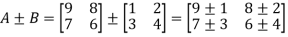
2. Scalar multiplication of matrix:
In this we multiply the scalar or constant with each element of the matrix.
Example: 
3. Multiplication of matrices: Two matrices can be multiplied only if they are conformal i.e. the number of column of first matrix is equal to the number rows of the second matrix.
Example: 
Then 
4. Power of Matrices: If A is A square matrix then

 and so on.
If  where A is square matrix then it is said to be idempotent.
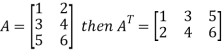
5. Transpose of a matrix: The matrix obtained from any given matrix A , by interchanging rows and columns is called the transpose of A and is denoted by 

The transpose of matrix  Also
Also 
Note: 
6. Trace of a matrix-
Suppose A be a square matrix, then the sum of its diagonal elements is known as trace of the matrix.
Example- If we have a matrix A-

Then the trace of A = 0 + 2 + 4 = 6
Rank of a matrix by echelon form-
The rank of a matrix (r) can be defined as –
1. It has atleast one non-zero minor of order r.
2. Every minor of A of order higher than r is zero.
Example: Find the rank of a matrix M by echelon form.
M = 
Sol. First we will convert the matrix M into echelon form,
M = 
Apply,  , we get
M = 
Apply  , we get
M = 
Apply 
M = 
We can see that, in this echelon form of matrix, the number of non – zero rows is 3.
So that the rank of matrix X will be 3.
Example: Find the rank of a matrix A by echelon form.
A = 
Sol. Convert the matrix A into echelon form,
A = 
Apply 
A = 
Apply  , we get
A = 
Apply  , we get
A = 
Apply  ,
,
A = 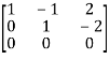
Apply  ,
,
A = 
Therefore the rank of the matrix will be 2.
Example: Find the rank of the following matrices by echelon form?
Let A = 
Applying 
A 
Applying 
A 
Applying 
A 
Applying 
A 
It is clear that minor of order 3 vanishes but minor of order 2 exists as 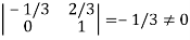
Hence rank of a given matrix A is 2 denoted by 
2. 
Let A = 
Applying 

Applying 

Applying 

The minor of order 3 vanishes but minor of order 2 non zero as 
Hence the rank of matrix A is 2 denoted by 
3. 
Let A = 
Apply 

Apply 

Apply 

It is clear that the minor of order 3 vanishes where as the minor of order 2 is non zero as 
Hence the rank of given matrix is 2 i.e. 
Characteristic roots and vectors (Eigen values & Eigen vectors)
Suppose we have A =  be an n × n matrix , then
Characteristic equation- The equation | = 0 is called the characteristic equation of A, where |
 is called characteristic matrix of A. Here I is the identity matrix.
The determinant | is called the characteristic polynomial of A.
Characteristic roots-the roots of the characteristic equation are known as characteristic roots or Eigen values or characteristic values.
Important notes on characteristic roots-
1. The characteristic roots of the matrix ‘A’ and its transpose A’ are always same.
2. If A and B are two matrices of the same type and B is invertible then the matrices A and  have the same characteristic roots.
3. If A and B are two square matrices which are invertible then AB and BA have the same characteristic roots.
4. Zero is a characteristic root of a matrix if and only if the given matrix is singular.
Solved examples to find characteristics equation-
Example-1: Find the characteristic equation of the matrix A:
A = 
Sol. The characteristic equation will be-
| = 0
= 0
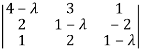 = 0
= 0
On solving the determinant, we get
(4-
Or 
On solving we get,

Which is the characteristic equation of matrix A.
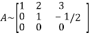
Example-2: Find the characteristic equation and characteristic roots of the matrix A:
A = 
Sol. We know that the characteristic equation of the matrix A will be-
| = 0
= 0
So that matrix A becomes,
 = 0
= 0
Which gives , on solving
(1- = 0
= 0
Or 
Or (
Which is the characteristic equation of matrix A.
The characteristic roots will be,
( (
(
(
(
Values of  are-
are-

These are the characteristic roots of matrix A.
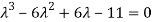
Example-3: Find the characteristic equation and characteristic roots of the matrix A:
A = 
Sol. We know that, the characteristic equation is-
| = 0
= 0
 = 0
= 0
Which gives,
(1-
Characteristic roots are- 
Eigen values and Eigen vectors-
Let A is a square matrix of order n. The equation formed by

Where I is an identity matrix of order n and  is unknown. It is called characteristic equation of the matrix A.

The values of the  are called the root of the characteristic equation, they are also known as characteristics roots or latent root or Eigen values of the matrix A.
Corresponding to each Eigen value there exist vectors X,

Called the characteristics vectors or latent vectors or Eigen vectors of the matrix A.
Note: Corresponding to distinct Eigen value we get distinct Eigen vectors but in case of repeated Eigen values we can have or not linearly independent Eigen vectors.
If  is Eigen vectors corresponding to Eigen value
  then
then  is also Eigen vectors for scalar c.
Properties of Eigen Values:
- The sum of the principal diagonal element of the matrix is equal to the sum of the all Eigen values of the matrix.
Let A be a matrix of order 3 then 
2. The determinant of the matrix A is equal to the product of the all Eigen values of the matrix then  .
.
3. If  is the Eigen value of the matrix A then 1/
 is the Eigen value of the
  .
.
4. If  is the Eigen value of an orthogonal matrix, then 1/
 is also its Eigen value.
5. If  are the Eigen values of the matrix A then
  has the Eigen values
  .
.
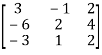
Example1: Find the sum and the product of the Eigen values of  ?
?
Sol. The sum of Eigen values = the sum of the diagonal elements
 =1+(-1)=0
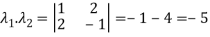
The product of the Eigen values is the determinant of the matrix

On solving above equations we get 
Example2: Find out the Eigen values and Eigen vectors of  ?
?
Sol. The Characteristics equation is given by 


Or 
Hence the Eigen values are 0,0 and 3.
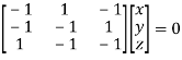
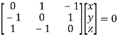
The Eigen vector corresponding to Eigen value  is
is

Where X is the column matrix of order 3 i.e.

This implies that 
Here number of unknowns are 3 and number of equation is 1.
Hence we have (3-1)=2 linearly independent solutions.
Let 
Thus the Eigen vectors corresponding to the Eigen value  are (-1,1,0) and (-2,1,1).
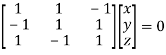
The Eigen vector corresponding to Eigen value  is
is

Where X is the column matrix of order 3 i.e.
This implies that 


Taking last two equations we get

Or 
Thus the Eigen vectors corresponding to the Eigen value  are (3,3,3).
Hence the three Eigen vectors obtained are (-1,1,0), (-2,1,1) and (3,3,3).
Example3: Find out the Eigen values and Eigen vectors of 
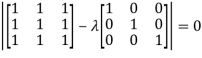
Sol. Let A =
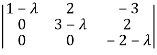
The characteristics equation of A is  .
.


Or 
Or 
Or 
Or 
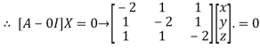
The Eigen vector corresponding to Eigen value  is
is

Where X is the column matrix of order 3 i.e.

Or 


On solving we get 
Thus the Eigen vectors corresponding to the Eigen value  is (1,1,1).
The Eigen vector corresponding to Eigen value  is
is

Where X is the column matrix of order 3 i.e.

Or 


On solving  or
or  .
.
Thus the Eigen vectors corresponding to the Eigen value  is (0,0,2).
The Eigen vector corresponding to Eigen value  is
is

Where X is the column matrix of order 3 i.e.

Or 


On solving we get  or
or  .
.
Thus the Eigen vectors corresponding to the Eigen value  is (2,2,2).
Hence three Eigen vectors are (1,1,1), (0,0,2) and (2,2,2).
Solution of homogeneous system of linear equations-
A system of linear equations of the form AX = O is said to be homogeneous , where A denotes the coefficients and of matrix and and O denotes the null vector.
Suppose the system of homogeneous linear equations is ,


It means ,
AX = O
Which can be written in the form of matrix as below,
Note- A system of homogeneous linear equations always has a solution if
1. r(A) = n then there will be trivial solution, where n is the number of unknown,
2. r(A) < n , then there will be an infinite number of solution.
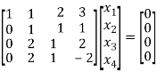
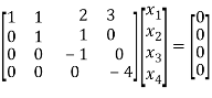
Example: Find the solution of the following homogeneous system of linear equations,


Sol. The given system of linear equations can be written in the form of matrix as follows,
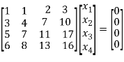
Apply the elementary row transformation,


 , we get,


 , we get

Here r(A) = 4, so that it has trivial solution,

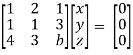
Example: Find out the value of ‘b’ in the system of homogenenous equations-
2x + y + 2z = 0
x + y + 3z = 0
4x + 3y + bz = 0
Which has
(1) trivial solution
(2) non-trivial solution
Sol. (1)
For trivial solution, we already know that the values of x , y and z will be zerp, so that ‘b’ can have any value.
Now for non-trivial solution-
(2)
Convert the system of equations into matrix form-
AX = O

Apply  respectively , we get the following resultant matrices
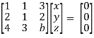

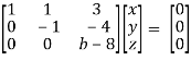
For non-trivial solutions , r(A) = 2 < n
b – 8 = 0
b = 8
Solution of non-homogeneous system of linear equations-
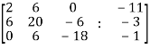
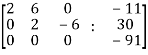
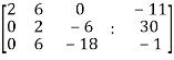
Example-1: check whether the following system of linear equations is consistent of not.
2x + 6y = -11
6x + 20y – 6z = -3
6y – 18z = -1
Sol. Write the above system of linear equations in augmented matrix form,
Apply  , we get

Apply 

Here the rank of C is 3 and the rank of A is 2
Therefore both ranks are not equal. So that the given system of linear equations is not consistent.
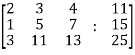
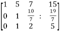
Example: Check the consistency and find the values of x , y and z of the following system of linear equations.
2x + 3y + 4z = 11
X + 5y + 7z = 15
3x + 11y + 13z = 25
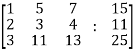
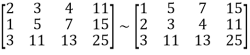
Sol. Re-write the system of equations in augmented matrix form.
C = [A,B]
That will be,

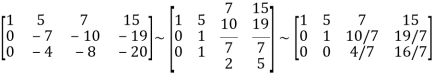
Apply 

Now apply ,
We get,
 ~
~ ~
~
Here rank of A = 3
And rank of C = 3, so that the system of equations is consistent,
So that we can solve the equations as below,
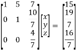
That gives,
x + 5y + 7z = 15 ……………..(1)
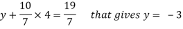
y + 10z/7 = 19/7 ………………(2)
4z/7 = 16/7 ………………….(3)
From eq. (3)
z = 4,
From 2,

From eq.(1), we get
x + 5(-3) + 7(4) = 15
That gives,
x = 2
Therefore the values of x , y , z are 2 , -3 , 4 respectively.
Consistency and inconsistency of linear systems
There are two types of linear equations-
1. Consistent 2. Inconsistent
Let’s understand about these two types of linear equations
Consistent –
If a system of equations has one or more than one solution, it is said be consistent.
There could be unique solution or infinite solution.
For example-
A system of linear equations-
2x + 4y = 9
x + y = 5
Has unique solution,
Where as,
A system of linear equations-
2x + y = 6
4x + 2y = 12
Has infinite solutions.
Inconsistent-
If a system of equations has no solution, then it is called inconsistent.
Consistency of a system of linear equations-
Suppose that a system of linear equations is given as-


This is the format as AX = B
Its augmented matrix is-
[A:B] = C
(1) consistent equations-
If Rank of A = Rank of C
Here, Rank of A = Rank of C = n ( no. Of unknown) – unique solution
And Rank of A = Rank of C = r , where r<n - infinite solutions
(2) inconsistent equations-
If Rank of A ≠ Rank of C
Example: Test the consistency of the following set of equations.
x1 + 2x2 + x3 = 2
3 x1 + x2 – 2x3 = 1
4x1 – 3x2 –x3 = 3
2x1 + 4x2 + 2x3 = 4
Sol. We can write the set of equations in matrix form:
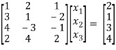
AX = B
We have augmented matrix C = [A:B]
~ 
~ 
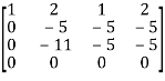
R2 R2 – 3 R1
R3 R3 – 4 R1
R4 R4 – 2 R1
~  R2 -1/5 R2
~  R3 R3 + 11 R2
~  R3 1/6 R3
Here we know that,
Number of non-zero rows = Rank of matrix
R(C) = R(A) = 3
Hence the given system is consistent and has unique solution.
Example: test the consistency:
2x + 3y + 4z = 11 , x + 5y + 7z = 15 , 3x + 11y + 13z = 25
Sol. Here augmented matrix is given by,
C = [A:B]
 R1 ↔ R2
R2 R2 – 2R1, R3 R3 – 3R1, R2 - 1/7 R2 , R3 - ¼ R3 , R3 R3 – R2

We notice here,
Rank of A= Rank of C = 3
Hence we can say that the system is consistent.
Linear dependence-
A set of n – vectors. x1, x2, …….., xr is said to be linearly dependent if there exist scalars. k1, k2, …….,kr not all zero such that
k1 + x2k2 + …………….. + xrkr = 0 … (1)
Linear independence-
A set of r vectors x1, x2, ………….,xr is said to be linearly independent if there exist scalars k1, k2, …………, kr all zero such that
x1 k1 + x2 k2 + …….. + xrkr = 0
Important notes-
- Equation (1) is known as a vector equation.
- If the vector equation has non – zero solution i.e. k1, k2, ….,kr not all zero. Then the vector x1, x2, ……….xr are said to be linearly dependent.
- If the vector equation has only trivial solution i.e.
k1 = k2 = …….=kr = 0. Then the vector x1, x2, ……,xr are said to linearly independent.
Linear combination-
A vector x can be written in the form.
x = x1 k1 + x2 k2 + ……….+xrkr
Where k1, k2, ………….., kr are scalars, then X is called linear combination of x1, x2, ……, xr.
Definition of linear transformation:
Suppose U(F) and V(F) are two vector spaces, then a mapping  is called a linear transformation of U into V, if:
1. 
2. 
It is also called homomorphism.
Kernel(null space) of a linear transformation-
Let f be a linear transformation of a vector space U(F) into a vector space V(F).
The kernel W of f is defined as-

The kernel W of f is a subset of U consisting of those elements of U which are mapped under f onto the zero vector V.
Since f(0) = 0, therefore atleast 0 belong to W. So that W is not empty.
Another definition of null space and range:
Let V and W be vector spaces, and let T: V → W be linear. We define the null space (or kernel) N(T) of T to be the set of all vectors x in V such that T(x) = 0; that is, N(T) = {x ∈ V: T(x) = 0 }.
We define the range (or image) R(T) of T to be the subset of W consisting of all images (under T) of vectors in V; that is, R(T) = {T(x) : x ∈ V}.
Example: The mapping  defined by-

Is a linear transformation  .
.
What is the kernel of this linear transformation.
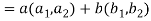
Sol. Let  be any two elements of
Let a, b be any two elements of F.
We have
 (
(


 =
= 

So that f is a linear transformation.
To show that f is onto  . Let
. Let  be any elements
  .
.
Then  and we have
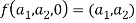
So that f is onto 
Therefore f is homomorphism of  onto
onto  .
.
If W is the kernel of this homomorphism then 
We have
∀
Also if  then
then 
Implies 
Therefore 
Hence W is the kernel of f.
Theorem: Let V and W be vector spaces and T: V → W be linear. Then N(T) and R(T) are subspaces of V and W, respectively.
Proof:
Here we will use the symbols 0 V and 0W to denote the zero vectors of V and W, respectively.
Since T(0 V) = 0W, we have that 0 V ∈ N(T). Let x, y ∈ N(T) and c ∈ F.
Then T(x + y) = T(x)+T(y) = 0W+0W = 0W, and T(c x) = c T(x) = c0W = 0W. Hence x + y ∈ N(T) and c x ∈ N(T), so that N(T) is a subspace of V. Because T(0 V) = 0W, we have that 0W ∈ R(T). Now let x, y ∈ R(T) and c ∈ F. Then there exist v and w in V such that T(v) = x and T(w) = y. So T(v + w) = T(v)+T(w) = x + y, and T(c v) = c T(v) = c x. Thus x+ y ∈ R(T) and c x ∈ R(T), so R(T) is a subspace of W.
Results:
- A set of two or more vectors are said to be linearly dependent if at least one vector can be written as a linear combination of the other vectors.
- A set of two or more vector are said to be linearly independent then no vector can be expressed as linear combination of the other vectors.
Matrix representation of a linear transformation
Linear transformation
Let V and U be vector spaces over the same field K. A mapping F : V  U is called a linear mapping or linear transformation if it satisfies the following two conditions:
(1) For any vectors v; w  V, F(v + w) = F(v) + F(w)
(2) For any scalar k and vector v  V, F(kv) = k F(v)
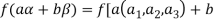
Now for any scalars a, b  K and any vector v, w
  V, we obtain
F (av + bw) = F(av) + F(bw) = a F(v) + b F(w)
Matrix representation of a linear transformation
Ordered basis- Let V be a finite-dimensional vector space. An ordered basis for V is a basis for V endowed with a specific order that is,
An ordered basis for V is a finite sequence of linearly independent vectors in V that generates V.
Definition:
Let  = {
= { ,
, , . . . ,
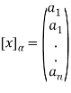
  } be an ordered basis for a finitedimensional vector space V. For x ∈ V, let
  ,
,  , . . . ,
 be the unique scalars such that

We define the coordinate vector of x relative to  , we denote it by
Example: let  given by

Let  be the standard ordered bases for
  , respectively. Now

And

Hence
If we suppose  , then

Example:  be the linear operator defined by F(x, y) = (2x + 3y, 4x – 5y).
Find the matrix representation of F relative to the basis S = {  } = {(1, 2), (2, 5)}
(1) First find F( , and then write it as a linear combination of the basis vectors
  and
and  . (For notational convenience, we use column vectors.) We have
And
X + 2y = 8
2x + 5y = -6
Solve the system to obtain x = 52, y =-22. Hence,

Now

X + 2y = 19
2x + 5y = -17
Solve the system to obtain x = 129, y =-55. Hence,

Now write the coordinates of  and
and  as columns to obtain the matrix

Steps to find Matrix Representations:
The input is a linear operator T on a vector space V and a basis S = { of V. The output is the matrix representation
Step 0- Find a formula for the coordinates of an arbitrary vector relative to the basis S.
Step 1- Repeat for each basis vector  in S:
in S:
(a) Find T( .
.
(b) Write T( as a linear combination of the basis vectors
Step 2- Form the matrix whose columns are the coordinate vectors in Step 1(b).
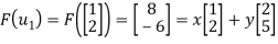
Example:  be the linear operator defined by F(x, y) = (2x + 3y, 4x – 5y).
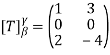
Find the matrix representation  of F relative to the basis S = {
  } = {(1, -2), (2, -5)}
Sol:
Step 0 - First find the coordinates of  relative to the basis S. We have

Or


Solving for x and y in terms of a and b yields x = 5a + 2b, y = -2a – b, thus

Step 1- Now we find  and write it as a linear combination of
  and
and  using the above formula for (a, b). And then we repeat the process for
  . We have


Step 2- Now, we write the coordinates of  and
and  as columns to obtain the required matrix:

Key takeaways:
- V be a finite-dimensional vector space. An ordered basis for V is a basis for V endowed with a specific order
- We define the coordinate vector of x relative to
 , we denote it by

References:
- E. Kreyszig, “Advanced Engineering Mathematics”, John Wiley & Sons, 2006.
- P. G. Hoel, S. C. Port And C. J. Stone, “Introduction To Probability Theory”, Universal Book Stall, 2003.
- S. Ross, “A First Course in Probability”, Pearson Education India, 2002.
- W. Feller, “An Introduction To Probability Theory and Its Applications”, Vol. 1, Wiley, 1968.
- N.P. Bali and M. Goyal, “A Text Book of Engineering Mathematics”, Laxmi Publications, 2010.
- B.S. Grewal, “Higher Engineering Mathematics”, Khanna Publishers, 2000.
Unit - 5
Linear Equations and Matrix Theory
Introduction:
Matrices has wide range of applications in various disciplines such as chemistry, Biology, Engineering, Statistics, economics, etc.
Matrices play an important role in computer science also.
Matrices are widely used to solving the system of linear equations, system of linear differential equations and non-linear differential equations.
First time the matrices were introduced by Cayley in 1860.
Definition-
A matrix is a rectangular arrangement of the numbers.
These numbers inside the matrix are known as elements of the matrix.
A matrix ‘A’ is expressed as-

The vertical elements are called columns and the horizontal elements are rows of the matrix.
The order of matrix A is m by n or (m× n)
Notation of a matrix-
A matrix ‘A’ is denoted as-
A = 
Where, i = 1, 2, …….,m and j = 1,2,3,…….n
Here ‘i’ denotes row and ‘j’ denotes column.
Types of matrices-
1. Rectangular matrix-
A matrix in which the number of rows is not equal to the number of columns, are called rectangular matrix.
Example:
A = 
The order of matrix A is 2×3 , that means it has two rows and three columns.
Matrix A is a rectangular matrix.
2. Square matrix-
A matrix which has equal number of rows and columns, is called square matrix.
Example:
A = 
The order of matrix A is 3 ×3 , that means it has three rows and three columns.
Matrix A is a square matrix.
3. Row matrix-
A matrix with a single row and any number of columns is called row matrix.
Example:
A = 
4. Column matrix-
A matrix with a single column and any number of rows is called row matrix.
Example:
A = 
5. Null matrix (Zero matrix)-
A matrix in which each element is zero, then it is called null matrix or zero matrix and denoted by O
Example:
A = 
6. Diagonal matrix-
A matrix is said to be diagonal matrix if all the elements except principal diagonal are zero
The diagonal matrix always follows- 
Example:
A = 
7. Scalar matrix-
A diagonal matrix in which all the diagonal elements are equal to a scalar, is called scalar matrix.
Example-
A = 
8. Identity matrix-
A diagonal matrix is said to be an identity matrix if its each element of diagonal is unity or 1.
It is denoted by – ‘I’
I = 
9. Triangular matrix-
If every element above or below the leading diagonal of a square matrix is zero, then the matrix is known as a triangular matrix.
There are two types of triangular matrices-
(a) Lower triangular matrix-
If all the elements below the leading diagonal of a square matrix are zero, then it is called lower triangular matrix.
Example:
A = 
(b) Upper triangular matrix-
If all the elements above the leading diagonal of a square matrix are zero, then it is called lower triangular matrix.
Example-
A = 
Algebra on Matrices:
- Addition and subtraction of matrices:
Addition and subtraction of matrices is possible if and only if they are of same order.
We add or subtract the corresponding elements of the matrices.
Example: 
2. Scalar multiplication of matrix:
In this we multiply the scalar or constant with each element of the matrix.
Example: 
3. Multiplication of matrices: Two matrices can be multiplied only if they are conformal i.e. the number of column of first matrix is equal to the number rows of the second matrix.
Example: 
Then 
4. Power of Matrices: If A is A square matrix then

 and so on.
If  where A is square matrix then it is said to be idempotent.
5. Transpose of a matrix: The matrix obtained from any given matrix A , by interchanging rows and columns is called the transpose of A and is denoted by 

The transpose of matrix 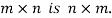 Also
Also 
Note: 
6. Trace of a matrix-
Suppose A be a square matrix, then the sum of its diagonal elements is known as trace of the matrix.
Example- If we have a matrix A-

Then the trace of A = 0 + 2 + 4 = 6
Rank of a matrix by echelon form-
The rank of a matrix (r) can be defined as –
1. It has atleast one non-zero minor of order r.
2. Every minor of A of order higher than r is zero.
Example: Find the rank of a matrix M by echelon form.
M = 
Sol. First we will convert the matrix M into echelon form,
M = 
Apply,  , we get
M = 
Apply  , we get
M = 
Apply 
M = 
We can see that, in this echelon form of matrix, the number of non – zero rows is 3.
So that the rank of matrix X will be 3.
Example: Find the rank of a matrix A by echelon form.
A = 
Sol. Convert the matrix A into echelon form,
A = 
Apply 
A = 
Apply  , we get
A = 
Apply  , we get
A = 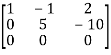
Apply  ,
,
A = 
Apply  ,
,
A = 
Therefore the rank of the matrix will be 2.
Example: Find the rank of the following matrices by echelon form?

Let A = 
Applying 
A 
Applying 
A 
Applying 
A 
Applying 
A 
It is clear that minor of order 3 vanishes but minor of order 2 exists as 
Hence rank of a given matrix A is 2 denoted by 
2. 
Let A = 
Applying 

Applying 

Applying 

The minor of order 3 vanishes but minor of order 2 non zero as 
Hence the rank of matrix A is 2 denoted by 
3. 
Let A = 
Apply 

Apply 

Apply 
It is clear that the minor of order 3 vanishes where as the minor of order 2 is non zero as 
Hence the rank of given matrix is 2 i.e. 
Characteristic roots and vectors (Eigen values & Eigen vectors)
Suppose we have A =  be an n × n matrix , then
Characteristic equation- The equation | = 0 is called the characteristic equation of A, where |
 is called characteristic matrix of A. Here I is the identity matrix.
The determinant | is called the characteristic polynomial of A.
Characteristic roots-the roots of the characteristic equation are known as characteristic roots or Eigen values or characteristic values.
Important notes on characteristic roots-
1. The characteristic roots of the matrix ‘A’ and its transpose A’ are always same.
2. If A and B are two matrices of the same type and B is invertible then the matrices A and  have the same characteristic roots.
3. If A and B are two square matrices which are invertible then AB and BA have the same characteristic roots.
4. Zero is a characteristic root of a matrix if and only if the given matrix is singular.
Solved examples to find characteristics equation-
Example-1: Find the characteristic equation of the matrix A:
A = 
Sol. The characteristic equation will be-
| = 0
= 0
 = 0
= 0
On solving the determinant, we get
(4-
Or 
On solving we get,

Which is the characteristic equation of matrix A.
Example-2: Find the characteristic equation and characteristic roots of the matrix A:
A = 
Sol. We know that the characteristic equation of the matrix A will be-
| = 0
= 0
So that matrix A becomes,
 = 0
= 0
Which gives , on solving
(1- = 0
= 0
Or 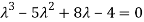
Or (
Which is the characteristic equation of matrix A.
The characteristic roots will be,
( (
(
(
(
Values of  are-
are-

These are the characteristic roots of matrix A.
Example-3: Find the characteristic equation and characteristic roots of the matrix A:
A = 
Sol. We know that, the characteristic equation is-
| = 0
= 0
 = 0
= 0
Which gives,
(1-
Characteristic roots are- 
Eigen values and Eigen vectors-
Let A is a square matrix of order n. The equation formed by

Where I is an identity matrix of order n and  is unknown. It is called characteristic equation of the matrix A.

The values of the  are called the root of the characteristic equation, they are also known as characteristics roots or latent root or Eigen values of the matrix A.
Corresponding to each Eigen value there exist vectors X,

Called the characteristics vectors or latent vectors or Eigen vectors of the matrix A.
Note: Corresponding to distinct Eigen value we get distinct Eigen vectors but in case of repeated Eigen values we can have or not linearly independent Eigen vectors.
If  is Eigen vectors corresponding to Eigen value
  then
then  is also Eigen vectors for scalar c.
Properties of Eigen Values:
- The sum of the principal diagonal element of the matrix is equal to the sum of the all Eigen values of the matrix.
Let A be a matrix of order 3 then 
2. The determinant of the matrix A is equal to the product of the all Eigen values of the matrix then  .
.
3. If  is the Eigen value of the matrix A then 1/
 is the Eigen value of the
  .
.
4. If  is the Eigen value of an orthogonal matrix, then 1/
 is also its Eigen value.
5. If  are the Eigen values of the matrix A then
  has the Eigen values
  .
.
Example1: Find the sum and the product of the Eigen values of  ?
?
Sol. The sum of Eigen values = the sum of the diagonal elements
 =1+(-1)=0
The product of the Eigen values is the determinant of the matrix
On solving above equations we get 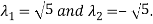
Example2: Find out the Eigen values and Eigen vectors of  ?
?
Sol. The Characteristics equation is given by 


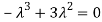
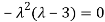
Or 
Hence the Eigen values are 0,0 and 3.
The Eigen vector corresponding to Eigen value  is
is

Where X is the column matrix of order 3 i.e.
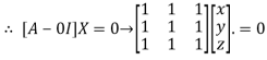
This implies that 
Here number of unknowns are 3 and number of equation is 1.
Hence we have (3-1)=2 linearly independent solutions.
Let 
Thus the Eigen vectors corresponding to the Eigen value  are (-1,1,0) and (-2,1,1).
The Eigen vector corresponding to Eigen value  is
is

Where X is the column matrix of order 3 i.e.

This implies that 


Taking last two equations we get

Or 
Thus the Eigen vectors corresponding to the Eigen value  are (3,3,3).
Hence the three Eigen vectors obtained are (-1,1,0), (-2,1,1) and (3,3,3).
Example3: Find out the Eigen values and Eigen vectors of 
Sol. Let A =
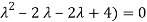
The characteristics equation of A is  .
.

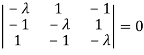
Or 
Or 
Or 
Or 
The Eigen vector corresponding to Eigen value  is
is

Where X is the column matrix of order 3 i.e.

Or 


On solving we get 
Thus the Eigen vectors corresponding to the Eigen value  is (1,1,1).
The Eigen vector corresponding to Eigen value  is
is

Where X is the column matrix of order 3 i.e.
Or 


On solving  or
or  .
.
Thus the Eigen vectors corresponding to the Eigen value  is (0,0,2).
The Eigen vector corresponding to Eigen value  is
is

Where X is the column matrix of order 3 i.e.
Or 


On solving we get  or
or  .
.
Thus the Eigen vectors corresponding to the Eigen value  is (2,2,2).
Hence three Eigen vectors are (1,1,1), (0,0,2) and (2,2,2).
Solution of homogeneous system of linear equations-
A system of linear equations of the form AX = O is said to be homogeneous , where A denotes the coefficients and of matrix and and O denotes the null vector.
Suppose the system of homogeneous linear equations is ,


It means ,
AX = O
Which can be written in the form of matrix as below,

Note- A system of homogeneous linear equations always has a solution if
1. r(A) = n then there will be trivial solution, where n is the number of unknown,
2. r(A) < n , then there will be an infinite number of solution.
Example: Find the solution of the following homogeneous system of linear equations,


Sol. The given system of linear equations can be written in the form of matrix as follows,

Apply the elementary row transformation,


 , we get,

 , we get

Here r(A) = 4, so that it has trivial solution,

Example: Find out the value of ‘b’ in the system of homogenenous equations-
2x + y + 2z = 0
x + y + 3z = 0
4x + 3y + bz = 0
Which has
(1) trivial solution
(2) non-trivial solution
Sol. (1)
For trivial solution, we already know that the values of x , y and z will be zerp, so that ‘b’ can have any value.
Now for non-trivial solution-
(2)
Convert the system of equations into matrix form-
AX = O

Apply  respectively , we get the following resultant matrices


For non-trivial solutions , r(A) = 2 < n
b – 8 = 0
b = 8
Solution of non-homogeneous system of linear equations-
Example-1: check whether the following system of linear equations is consistent of not.
2x + 6y = -11
6x + 20y – 6z = -3
6y – 18z = -1
Sol. Write the above system of linear equations in augmented matrix form,

Apply  , we get

Apply 
Here the rank of C is 3 and the rank of A is 2
Therefore both ranks are not equal. So that the given system of linear equations is not consistent.
Example: Check the consistency and find the values of x , y and z of the following system of linear equations.
2x + 3y + 4z = 11
X + 5y + 7z = 15
3x + 11y + 13z = 25
Sol. Re-write the system of equations in augmented matrix form.
C = [A,B]
That will be,
Apply 
Now apply ,
We get,
 ~
~ ~
~
Here rank of A = 3
And rank of C = 3, so that the system of equations is consistent,
So that we can solve the equations as below,

That gives,
x + 5y + 7z = 15 ……………..(1)
y + 10z/7 = 19/7 ………………(2)
4z/7 = 16/7 ………………….(3)
From eq. (3)
z = 4,
From 2,

From eq.(1), we get
x + 5(-3) + 7(4) = 15
That gives,
x = 2
Therefore the values of x , y , z are 2 , -3 , 4 respectively.
Consistency and inconsistency of linear systems
There are two types of linear equations-
1. Consistent 2. Inconsistent
Let’s understand about these two types of linear equations
Consistent –
If a system of equations has one or more than one solution, it is said be consistent.
There could be unique solution or infinite solution.
For example-
A system of linear equations-
2x + 4y = 9
x + y = 5
Has unique solution,
Where as,
A system of linear equations-
2x + y = 6
4x + 2y = 12
Has infinite solutions.
Inconsistent-
If a system of equations has no solution, then it is called inconsistent.
Consistency of a system of linear equations-
Suppose that a system of linear equations is given as-


This is the format as AX = B
Its augmented matrix is-
[A:B] = C
(1) consistent equations-
If Rank of A = Rank of C
Here, Rank of A = Rank of C = n ( no. Of unknown) – unique solution
And Rank of A = Rank of C = r , where r<n - infinite solutions
(2) inconsistent equations-
If Rank of A ≠ Rank of C
Example: Test the consistency of the following set of equations.
x1 + 2x2 + x3 = 2
3 x1 + x2 – 2x3 = 1
4x1 – 3x2 –x3 = 3
2x1 + 4x2 + 2x3 = 4
Sol. We can write the set of equations in matrix form:

AX = B
We have augmented matrix C = [A:B]
~ 
~ 
R2 R2 – 3 R1
R3 R3 – 4 R1
R4 R4 – 2 R1
~  R2 -1/5 R2
~  R3 R3 + 11 R2
~  R3 1/6 R3
Here we know that,
Number of non-zero rows = Rank of matrix
R(C) = R(A) = 3
Hence the given system is consistent and has unique solution.
Example: test the consistency:
2x + 3y + 4z = 11 , x + 5y + 7z = 15 , 3x + 11y + 13z = 25
Sol. Here augmented matrix is given by,
C = [A:B]
 R1 ↔ R2
R2 R2 – 2R1, R3 R3 – 3R1, R2 - 1/7 R2 , R3 - ¼ R3 , R3 R3 – R2

We notice here,
Rank of A= Rank of C = 3
Hence we can say that the system is consistent.
Linear dependence-
A set of n – vectors. x1, x2, …….., xr is said to be linearly dependent if there exist scalars. k1, k2, …….,kr not all zero such that
k1 + x2k2 + …………….. + xrkr = 0 … (1)
Linear independence-
A set of r vectors x1, x2, ………….,xr is said to be linearly independent if there exist scalars k1, k2, …………, kr all zero such that
x1 k1 + x2 k2 + …….. + xrkr = 0
Important notes-
- Equation (1) is known as a vector equation.
- If the vector equation has non – zero solution i.e. k1, k2, ….,kr not all zero. Then the vector x1, x2, ……….xr are said to be linearly dependent.
- If the vector equation has only trivial solution i.e.
k1 = k2 = …….=kr = 0. Then the vector x1, x2, ……,xr are said to linearly independent.
Linear combination-
A vector x can be written in the form.
x = x1 k1 + x2 k2 + ……….+xrkr
Where k1, k2, ………….., kr are scalars, then X is called linear combination of x1, x2, ……, xr.
Definition of linear transformation:
Suppose U(F) and V(F) are two vector spaces, then a mapping  is called a linear transformation of U into V, if:
1. 
2. 
It is also called homomorphism.
Kernel(null space) of a linear transformation-
Let f be a linear transformation of a vector space U(F) into a vector space V(F).
The kernel W of f is defined as-

The kernel W of f is a subset of U consisting of those elements of U which are mapped under f onto the zero vector V.
Since f(0) = 0, therefore atleast 0 belong to W. So that W is not empty.
Another definition of null space and range:
Let V and W be vector spaces, and let T: V → W be linear. We define the null space (or kernel) N(T) of T to be the set of all vectors x in V such that T(x) = 0; that is, N(T) = {x ∈ V: T(x) = 0 }.
We define the range (or image) R(T) of T to be the subset of W consisting of all images (under T) of vectors in V; that is, R(T) = {T(x) : x ∈ V}.
Example: The mapping 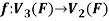 defined by-

Is a linear transformation  .
.
What is the kernel of this linear transformation.
Sol. Let  be any two elements of
Let a, b be any two elements of F.
We have
 (
(


 =
= 

So that f is a linear transformation.
To show that f is onto  . Let
. Let  be any elements
  .
.
Then  and we have
So that f is onto 
Therefore f is homomorphism of  onto
onto  .
.
If W is the kernel of this homomorphism then 
We have
∀
Also if  then
then 
Implies 
Therefore 
Hence W is the kernel of f.
Theorem: Let V and W be vector spaces and T: V → W be linear. Then N(T) and R(T) are subspaces of V and W, respectively.
Proof:
Here we will use the symbols 0 V and 0W to denote the zero vectors of V and W, respectively.
Since T(0 V) = 0W, we have that 0 V ∈ N(T). Let x, y ∈ N(T) and c ∈ F.
Then T(x + y) = T(x)+T(y) = 0W+0W = 0W, and T(c x) = c T(x) = c0W = 0W. Hence x + y ∈ N(T) and c x ∈ N(T), so that N(T) is a subspace of V. Because T(0 V) = 0W, we have that 0W ∈ R(T). Now let x, y ∈ R(T) and c ∈ F. Then there exist v and w in V such that T(v) = x and T(w) = y. So T(v + w) = T(v)+T(w) = x + y, and T(c v) = c T(v) = c x. Thus x+ y ∈ R(T) and c x ∈ R(T), so R(T) is a subspace of W.
Results:
- A set of two or more vectors are said to be linearly dependent if at least one vector can be written as a linear combination of the other vectors.
- A set of two or more vector are said to be linearly independent then no vector can be expressed as linear combination of the other vectors.
Matrix representation of a linear transformation
Linear transformation
Let V and U be vector spaces over the same field K. A mapping F : V  U is called a linear mapping or linear transformation if it satisfies the following two conditions:
(1) For any vectors v; w  V, F(v + w) = F(v) + F(w)
(2) For any scalar k and vector v  V, F(kv) = k F(v)
Now for any scalars a, b  K and any vector v, w
  V, we obtain
F (av + bw) = F(av) + F(bw) = a F(v) + b F(w)
Matrix representation of a linear transformation
Ordered basis- Let V be a finite-dimensional vector space. An ordered basis for V is a basis for V endowed with a specific order that is,
An ordered basis for V is a finite sequence of linearly independent vectors in V that generates V.
Definition:
Let  = {
= { ,
, , . . . ,
  } be an ordered basis for a finitedimensional vector space V. For x ∈ V, let
  ,
,  , . . . ,
 be the unique scalars such that

We define the coordinate vector of x relative to  , we denote it by

Example: let  given by

Let  be the standard ordered bases for
  , respectively. Now

And

Hence

If we suppose  , then

Example:  be the linear operator defined by F(x, y) = (2x + 3y, 4x – 5y).
Find the matrix representation of F relative to the basis S = {  } = {(1, 2), (2, 5)}
(1) First find F( , and then write it as a linear combination of the basis vectors
  and
and  . (For notational convenience, we use column vectors.) We have

And
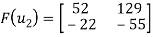
X + 2y = 8
2x + 5y = -6
Solve the system to obtain x = 52, y =-22. Hence,

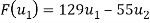
Now

X + 2y = 19
2x + 5y = -17
Solve the system to obtain x = 129, y =-55. Hence,
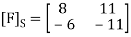
Now write the coordinates of  and
and  as columns to obtain the matrix
Steps to find Matrix Representations:
The input is a linear operator T on a vector space V and a basis S = { of V. The output is the matrix representation
Step 0- Find a formula for the coordinates of an arbitrary vector relative to the basis S.
Step 1- Repeat for each basis vector  in S:
in S:
(a) Find T( .
.
(b) Write T( as a linear combination of the basis vectors
Step 2- Form the matrix whose columns are the coordinate vectors in Step 1(b).
Example:  be the linear operator defined by F(x, y) = (2x + 3y, 4x – 5y).
Find the matrix representation  of F relative to the basis S = {
  } = {(1, -2), (2, -5)}
Sol:
Step 0 - First find the coordinates of  relative to the basis S. We have

Or


Solving for x and y in terms of a and b yields x = 5a + 2b, y = -2a – b, thus

Step 1- Now we find  and write it as a linear combination of
  and
and  using the above formula for (a, b). And then we repeat the process for
  . We have


Step 2- Now, we write the coordinates of  and
and  as columns to obtain the required matrix:
Key takeaways:
- V be a finite-dimensional vector space. An ordered basis for V is a basis for V endowed with a specific order
- We define the coordinate vector of x relative to
 , we denote it by

References:
- E. Kreyszig, “Advanced Engineering Mathematics”, John Wiley & Sons, 2006.
- P. G. Hoel, S. C. Port And C. J. Stone, “Introduction To Probability Theory”, Universal Book Stall, 2003.
- S. Ross, “A First Course in Probability”, Pearson Education India, 2002.
- W. Feller, “An Introduction To Probability Theory and Its Applications”, Vol. 1, Wiley, 1968.
- N.P. Bali and M. Goyal, “A Text Book of Engineering Mathematics”, Laxmi Publications, 2010.
- B.S. Grewal, “Higher Engineering Mathematics”, Khanna Publishers, 2000.
Unit - 5
Linear Equations and Matrix Theory
Unit - 5
Linear Equations and Matrix Theory
Unit - 5
Linear Equations and Matrix Theory
Unit - 5
Linear Equations and Matrix Theory
Unit - 5
Linear Equations and Matrix Theory
Introduction:
Matrices has wide range of applications in various disciplines such as chemistry, Biology, Engineering, Statistics, economics, etc.
Matrices play an important role in computer science also.
Matrices are widely used to solving the system of linear equations, system of linear differential equations and non-linear differential equations.
First time the matrices were introduced by Cayley in 1860.
Definition-
A matrix is a rectangular arrangement of the numbers.
These numbers inside the matrix are known as elements of the matrix.
A matrix ‘A’ is expressed as-

The vertical elements are called columns and the horizontal elements are rows of the matrix.
The order of matrix A is m by n or (m× n)
Notation of a matrix-
A matrix ‘A’ is denoted as-
A = 
Where, i = 1, 2, …….,m and j = 1,2,3,…….n
Here ‘i’ denotes row and ‘j’ denotes column.
Types of matrices-
1. Rectangular matrix-
A matrix in which the number of rows is not equal to the number of columns, are called rectangular matrix.
Example:
A = 
The order of matrix A is 2×3 , that means it has two rows and three columns.
Matrix A is a rectangular matrix.
2. Square matrix-
A matrix which has equal number of rows and columns, is called square matrix.
Example:
A = 
The order of matrix A is 3 ×3 , that means it has three rows and three columns.
Matrix A is a square matrix.
3. Row matrix-
A matrix with a single row and any number of columns is called row matrix.
Example:
A = 
4. Column matrix-
A matrix with a single column and any number of rows is called row matrix.
Example:
A = 
5. Null matrix (Zero matrix)-
A matrix in which each element is zero, then it is called null matrix or zero matrix and denoted by O
Example:
A = 
6. Diagonal matrix-
A matrix is said to be diagonal matrix if all the elements except principal diagonal are zero
The diagonal matrix always follows- 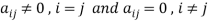
Example:
A = 
7. Scalar matrix-
A diagonal matrix in which all the diagonal elements are equal to a scalar, is called scalar matrix.
Example-
A = 
8. Identity matrix-
A diagonal matrix is said to be an identity matrix if its each element of diagonal is unity or 1.
It is denoted by – ‘I’
I = 
9. Triangular matrix-
If every element above or below the leading diagonal of a square matrix is zero, then the matrix is known as a triangular matrix.
There are two types of triangular matrices-
(a) Lower triangular matrix-
If all the elements below the leading diagonal of a square matrix are zero, then it is called lower triangular matrix.
Example:
A = 
(b) Upper triangular matrix-
If all the elements above the leading diagonal of a square matrix are zero, then it is called lower triangular matrix.
Example-
A = 
Algebra on Matrices:
- Addition and subtraction of matrices:
Addition and subtraction of matrices is possible if and only if they are of same order.
We add or subtract the corresponding elements of the matrices.
Example: 
2. Scalar multiplication of matrix:
In this we multiply the scalar or constant with each element of the matrix.
Example: 
3. Multiplication of matrices: Two matrices can be multiplied only if they are conformal i.e. the number of column of first matrix is equal to the number rows of the second matrix.
Example: 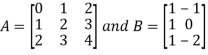
Then 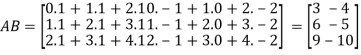
4. Power of Matrices: If A is A square matrix then

 and so on.
If  where A is square matrix then it is said to be idempotent.
5. Transpose of a matrix: The matrix obtained from any given matrix A , by interchanging rows and columns is called the transpose of A and is denoted by 
The transpose of matrix  Also
Also 
Note: 
6. Trace of a matrix-
Suppose A be a square matrix, then the sum of its diagonal elements is known as trace of the matrix.
Example- If we have a matrix A-

Then the trace of A = 0 + 2 + 4 = 6
Rank of a matrix by echelon form-
The rank of a matrix (r) can be defined as –
1. It has atleast one non-zero minor of order r.
2. Every minor of A of order higher than r is zero.
Example: Find the rank of a matrix M by echelon form.
M = 
Sol. First we will convert the matrix M into echelon form,
M = 
Apply,  , we get
M = 
Apply  , we get
M = 
Apply 
M = 
We can see that, in this echelon form of matrix, the number of non – zero rows is 3.
So that the rank of matrix X will be 3.
Example: Find the rank of a matrix A by echelon form.
A = 
Sol. Convert the matrix A into echelon form,
A = 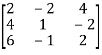
Apply 
A = 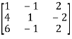
Apply 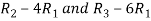 , we get
A = 
Apply  , we get
A = 
Apply  ,
,
A = 
Apply  ,
,
A = 
Therefore the rank of the matrix will be 2.
Example: Find the rank of the following matrices by echelon form?

Let A = 
Applying 
A 
Applying 
A 
Applying 
A 
Applying 
A 
It is clear that minor of order 3 vanishes but minor of order 2 exists as 
Hence rank of a given matrix A is 2 denoted by 
2. 
Let A = 
Applying 

Applying 

Applying 

The minor of order 3 vanishes but minor of order 2 non zero as 
Hence the rank of matrix A is 2 denoted by 
3. 
Let A = 
Apply 

Apply 

Apply 

It is clear that the minor of order 3 vanishes where as the minor of order 2 is non zero as 
Hence the rank of given matrix is 2 i.e. 
Characteristic roots and vectors (Eigen values & Eigen vectors)
Suppose we have A =  be an n × n matrix , then
Characteristic equation- The equation | = 0 is called the characteristic equation of A, where |
 is called characteristic matrix of A. Here I is the identity matrix.
The determinant | is called the characteristic polynomial of A.
Characteristic roots-the roots of the characteristic equation are known as characteristic roots or Eigen values or characteristic values.
Important notes on characteristic roots-
1. The characteristic roots of the matrix ‘A’ and its transpose A’ are always same.
2. If A and B are two matrices of the same type and B is invertible then the matrices A and  have the same characteristic roots.
3. If A and B are two square matrices which are invertible then AB and BA have the same characteristic roots.
4. Zero is a characteristic root of a matrix if and only if the given matrix is singular.
Solved examples to find characteristics equation-
Example-1: Find the characteristic equation of the matrix A:
A = 
Sol. The characteristic equation will be-
| = 0
= 0
 = 0
= 0
On solving the determinant, we get
(4-
Or 
On solving we get,
Which is the characteristic equation of matrix A.
Example-2: Find the characteristic equation and characteristic roots of the matrix A:
A = 
Sol. We know that the characteristic equation of the matrix A will be-
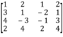
| = 0
= 0
So that matrix A becomes,
 = 0
= 0
Which gives , on solving
(1- = 0
= 0
Or 
Or (
Which is the characteristic equation of matrix A.
The characteristic roots will be,
( (
(
(
(
Values of  are-
are-

These are the characteristic roots of matrix A.
Example-3: Find the characteristic equation and characteristic roots of the matrix A:
A = 
Sol. We know that, the characteristic equation is-
| = 0
= 0
 = 0
= 0
Which gives,
(1-
Characteristic roots are- 
Eigen values and Eigen vectors-
Let A is a square matrix of order n. The equation formed by

Where I is an identity matrix of order n and  is unknown. It is called characteristic equation of the matrix A.

The values of the  are called the root of the characteristic equation, they are also known as characteristics roots or latent root or Eigen values of the matrix A.
Corresponding to each Eigen value there exist vectors X,

Called the characteristics vectors or latent vectors or Eigen vectors of the matrix A.
Note: Corresponding to distinct Eigen value we get distinct Eigen vectors but in case of repeated Eigen values we can have or not linearly independent Eigen vectors.
If  is Eigen vectors corresponding to Eigen value
  then
then  is also Eigen vectors for scalar c.
Properties of Eigen Values:
- The sum of the principal diagonal element of the matrix is equal to the sum of the all Eigen values of the matrix.
Let A be a matrix of order 3 then 
2. The determinant of the matrix A is equal to the product of the all Eigen values of the matrix then  .
.
3. If  is the Eigen value of the matrix A then 1/
 is the Eigen value of the
  .
.
4. If  is the Eigen value of an orthogonal matrix, then 1/
 is also its Eigen value.
5. If  are the Eigen values of the matrix A then
  has the Eigen values
  .
.
Example1: Find the sum and the product of the Eigen values of  ?
?
Sol. The sum of Eigen values = the sum of the diagonal elements
 =1+(-1)=0
The product of the Eigen values is the determinant of the matrix

On solving above equations we get 
Example2: Find out the Eigen values and Eigen vectors of  ?
?
Sol. The Characteristics equation is given by 


Or 
Hence the Eigen values are 0,0 and 3.
The Eigen vector corresponding to Eigen value  is
is

Where X is the column matrix of order 3 i.e.

This implies that 
Here number of unknowns are 3 and number of equation is 1.
Hence we have (3-1)=2 linearly independent solutions.
Let 
Thus the Eigen vectors corresponding to the Eigen value  are (-1,1,0) and (-2,1,1).
The Eigen vector corresponding to Eigen value  is
is

Where X is the column matrix of order 3 i.e.

This implies that 


Taking last two equations we get

Or 
Thus the Eigen vectors corresponding to the Eigen value  are (3,3,3).
Hence the three Eigen vectors obtained are (-1,1,0), (-2,1,1) and (3,3,3).
Example3: Find out the Eigen values and Eigen vectors of 
Sol. Let A =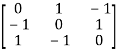
The characteristics equation of A is  .
.


Or 
Or 
Or 
Or 
The Eigen vector corresponding to Eigen value  is
is

Where X is the column matrix of order 3 i.e.
Or 


On solving we get 
Thus the Eigen vectors corresponding to the Eigen value  is (1,1,1).
The Eigen vector corresponding to Eigen value  is
is

Where X is the column matrix of order 3 i.e.

Or 


On solving  or
or  .
.
Thus the Eigen vectors corresponding to the Eigen value  is (0,0,2).
The Eigen vector corresponding to Eigen value  is
is

Where X is the column matrix of order 3 i.e.

Or 


On solving we get 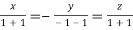 or
or  .
.
Thus the Eigen vectors corresponding to the Eigen value  is (2,2,2).
Hence three Eigen vectors are (1,1,1), (0,0,2) and (2,2,2).
Solution of homogeneous system of linear equations-
A system of linear equations of the form AX = O is said to be homogeneous , where A denotes the coefficients and of matrix and and O denotes the null vector.
Suppose the system of homogeneous linear equations is ,


It means ,
AX = O
Which can be written in the form of matrix as below,

Note- A system of homogeneous linear equations always has a solution if
1. r(A) = n then there will be trivial solution, where n is the number of unknown,
2. r(A) < n , then there will be an infinite number of solution.
Example: Find the solution of the following homogeneous system of linear equations,


Sol. The given system of linear equations can be written in the form of matrix as follows,

Apply the elementary row transformation,


 , we get,


 , we get
Here r(A) = 4, so that it has trivial solution,

Example: Find out the value of ‘b’ in the system of homogenenous equations-
2x + y + 2z = 0
x + y + 3z = 0
4x + 3y + bz = 0
Which has
(1) trivial solution
(2) non-trivial solution
Sol. (1)
For trivial solution, we already know that the values of x , y and z will be zerp, so that ‘b’ can have any value.
Now for non-trivial solution-
(2)
Convert the system of equations into matrix form-
AX = O
Apply  respectively , we get the following resultant matrices


For non-trivial solutions , r(A) = 2 < n
b – 8 = 0
b = 8
Solution of non-homogeneous system of linear equations-
Example-1: check whether the following system of linear equations is consistent of not.
2x + 6y = -11
6x + 20y – 6z = -3
6y – 18z = -1
Sol. Write the above system of linear equations in augmented matrix form,

Apply  , we get
Apply 

Here the rank of C is 3 and the rank of A is 2
Therefore both ranks are not equal. So that the given system of linear equations is not consistent.
Example: Check the consistency and find the values of x , y and z of the following system of linear equations.
2x + 3y + 4z = 11
X + 5y + 7z = 15
3x + 11y + 13z = 25
Sol. Re-write the system of equations in augmented matrix form.
C = [A,B]
That will be,

Apply 

Now apply ,
We get,
 ~
~ ~
~
Here rank of A = 3
And rank of C = 3, so that the system of equations is consistent,
So that we can solve the equations as below,

That gives,
x + 5y + 7z = 15 ……………..(1)
y + 10z/7 = 19/7 ………………(2)
4z/7 = 16/7 ………………….(3)
From eq. (3)
z = 4,
From 2,
From eq.(1), we get
x + 5(-3) + 7(4) = 15
That gives,
x = 2
Therefore the values of x , y , z are 2 , -3 , 4 respectively.
Consistency and inconsistency of linear systems
There are two types of linear equations-
1. Consistent 2. Inconsistent
Let’s understand about these two types of linear equations
Consistent –
If a system of equations has one or more than one solution, it is said be consistent.
There could be unique solution or infinite solution.
For example-
A system of linear equations-
2x + 4y = 9
x + y = 5
Has unique solution,
Where as,
A system of linear equations-
2x + y = 6
4x + 2y = 12
Has infinite solutions.
Inconsistent-
If a system of equations has no solution, then it is called inconsistent.
Consistency of a system of linear equations-
Suppose that a system of linear equations is given as-


This is the format as AX = B
Its augmented matrix is-
[A:B] = C
(1) consistent equations-
If Rank of A = Rank of C
Here, Rank of A = Rank of C = n ( no. Of unknown) – unique solution
And Rank of A = Rank of C = r , where r<n - infinite solutions
(2) inconsistent equations-
If Rank of A ≠ Rank of C
Example: Test the consistency of the following set of equations.
x1 + 2x2 + x3 = 2
3 x1 + x2 – 2x3 = 1
4x1 – 3x2 –x3 = 3
2x1 + 4x2 + 2x3 = 4
Sol. We can write the set of equations in matrix form:

AX = B
We have augmented matrix C = [A:B]
~ 
~ 
R2 R2 – 3 R1
R3 R3 – 4 R1
R4 R4 – 2 R1
~  R2 -1/5 R2
~  R3 R3 + 11 R2
~  R3 1/6 R3
Here we know that,
Number of non-zero rows = Rank of matrix
R(C) = R(A) = 3
Hence the given system is consistent and has unique solution.
Example: test the consistency:
2x + 3y + 4z = 11 , x + 5y + 7z = 15 , 3x + 11y + 13z = 25
Sol. Here augmented matrix is given by,
C = [A:B]
 R1 ↔ R2
R2 R2 – 2R1, R3 R3 – 3R1, R2 - 1/7 R2 , R3 - ¼ R3 , R3 R3 – R2
We notice here,
Rank of A= Rank of C = 3
Hence we can say that the system is consistent.
Linear dependence-
A set of n – vectors. x1, x2, …….., xr is said to be linearly dependent if there exist scalars. k1, k2, …….,kr not all zero such that
k1 + x2k2 + …………….. + xrkr = 0 … (1)
Linear independence-
A set of r vectors x1, x2, ………….,xr is said to be linearly independent if there exist scalars k1, k2, …………, kr all zero such that
x1 k1 + x2 k2 + …….. + xrkr = 0
Important notes-
- Equation (1) is known as a vector equation.
- If the vector equation has non – zero solution i.e. k1, k2, ….,kr not all zero. Then the vector x1, x2, ……….xr are said to be linearly dependent.
- If the vector equation has only trivial solution i.e.
k1 = k2 = …….=kr = 0. Then the vector x1, x2, ……,xr are said to linearly independent.
Linear combination-
A vector x can be written in the form.
x = x1 k1 + x2 k2 + ……….+xrkr
Where k1, k2, ………….., kr are scalars, then X is called linear combination of x1, x2, ……, xr.
Definition of linear transformation:
Suppose U(F) and V(F) are two vector spaces, then a mapping  is called a linear transformation of U into V, if:
1. 
2. 
It is also called homomorphism.
Kernel(null space) of a linear transformation-
Let f be a linear transformation of a vector space U(F) into a vector space V(F).
The kernel W of f is defined as-

The kernel W of f is a subset of U consisting of those elements of U which are mapped under f onto the zero vector V.
Since f(0) = 0, therefore atleast 0 belong to W. So that W is not empty.
Another definition of null space and range:
Let V and W be vector spaces, and let T: V → W be linear. We define the null space (or kernel) N(T) of T to be the set of all vectors x in V such that T(x) = 0; that is, N(T) = {x ∈ V: T(x) = 0 }.
We define the range (or image) R(T) of T to be the subset of W consisting of all images (under T) of vectors in V; that is, R(T) = {T(x) : x ∈ V}.
Example: The mapping  defined by-

Is a linear transformation  .
.
What is the kernel of this linear transformation.
Sol. Let  be any two elements of
Let a, b be any two elements of F.
We have
 (
(


 =
= 

So that f is a linear transformation.
To show that f is onto  . Let
. Let  be any elements
  .
.
Then  and we have
So that f is onto 
Therefore f is homomorphism of  onto
onto  .
.
If W is the kernel of this homomorphism then 
We have
∀
Also if  then
then 
Implies 
Therefore 
Hence W is the kernel of f.
Theorem: Let V and W be vector spaces and T: V → W be linear. Then N(T) and R(T) are subspaces of V and W, respectively.
Proof:
Here we will use the symbols 0 V and 0W to denote the zero vectors of V and W, respectively.
Since T(0 V) = 0W, we have that 0 V ∈ N(T). Let x, y ∈ N(T) and c ∈ F.
Then T(x + y) = T(x)+T(y) = 0W+0W = 0W, and T(c x) = c T(x) = c0W = 0W. Hence x + y ∈ N(T) and c x ∈ N(T), so that N(T) is a subspace of V. Because T(0 V) = 0W, we have that 0W ∈ R(T). Now let x, y ∈ R(T) and c ∈ F. Then there exist v and w in V such that T(v) = x and T(w) = y. So T(v + w) = T(v)+T(w) = x + y, and T(c v) = c T(v) = c x. Thus x+ y ∈ R(T) and c x ∈ R(T), so R(T) is a subspace of W.
Results:
- A set of two or more vectors are said to be linearly dependent if at least one vector can be written as a linear combination of the other vectors.
- A set of two or more vector are said to be linearly independent then no vector can be expressed as linear combination of the other vectors.
Matrix representation of a linear transformation
Linear transformation
Let V and U be vector spaces over the same field K. A mapping F : V  U is called a linear mapping or linear transformation if it satisfies the following two conditions:
(1) For any vectors v; w  V, F(v + w) = F(v) + F(w)
(2) For any scalar k and vector v  V, F(kv) = k F(v)
Now for any scalars a, b  K and any vector v, w
  V, we obtain
F (av + bw) = F(av) + F(bw) = a F(v) + b F(w)
Matrix representation of a linear transformation
Ordered basis- Let V be a finite-dimensional vector space. An ordered basis for V is a basis for V endowed with a specific order that is,
An ordered basis for V is a finite sequence of linearly independent vectors in V that generates V.
Definition:
Let  = {
= { ,
, , . . . ,
  } be an ordered basis for a finitedimensional vector space V. For x ∈ V, let
  ,
,  , . . . ,
 be the unique scalars such that

We define the coordinate vector of x relative to  , we denote it by

Example: let  given by

Let  be the standard ordered bases for
  , respectively. Now

And

Hence

If we suppose  , then

Example:  be the linear operator defined by F(x, y) = (2x + 3y, 4x – 5y).
Find the matrix representation of F relative to the basis S = {  } = {(1, 2), (2, 5)}
(1) First find F( , and then write it as a linear combination of the basis vectors
  and
and  . (For notational convenience, we use column vectors.) We have

And
X + 2y = 8
2x + 5y = -6
Solve the system to obtain x = 52, y =-22. Hence,

Now

X + 2y = 19
2x + 5y = -17
Solve the system to obtain x = 129, y =-55. Hence,

Now write the coordinates of  and
and  as columns to obtain the matrix

Steps to find Matrix Representations:
The input is a linear operator T on a vector space V and a basis S = { of V. The output is the matrix representation
Step 0- Find a formula for the coordinates of an arbitrary vector relative to the basis S.
Step 1- Repeat for each basis vector  in S:
in S:
(a) Find T( .
.
(b) Write T( as a linear combination of the basis vectors
Step 2- Form the matrix whose columns are the coordinate vectors in Step 1(b).
Example:  be the linear operator defined by F(x, y) = (2x + 3y, 4x – 5y).
Find the matrix representation  of F relative to the basis S = {
  } = {(1, -2), (2, -5)}
Sol:
Step 0 - First find the coordinates of  relative to the basis S. We have

Or


Solving for x and y in terms of a and b yields x = 5a + 2b, y = -2a – b, thus

Step 1- Now we find  and write it as a linear combination of
  and
and  using the above formula for (a, b). And then we repeat the process for
  . We have


Step 2- Now, we write the coordinates of  and
and  as columns to obtain the required matrix:

Key takeaways:
- V be a finite-dimensional vector space. An ordered basis for V is a basis for V endowed with a specific order
- We define the coordinate vector of x relative to
 , we denote it by

References:
- E. Kreyszig, “Advanced Engineering Mathematics”, John Wiley & Sons, 2006.
- P. G. Hoel, S. C. Port And C. J. Stone, “Introduction To Probability Theory”, Universal Book Stall, 2003.
- S. Ross, “A First Course in Probability”, Pearson Education India, 2002.
- W. Feller, “An Introduction To Probability Theory and Its Applications”, Vol. 1, Wiley, 1968.
- N.P. Bali and M. Goyal, “A Text Book of Engineering Mathematics”, Laxmi Publications, 2010.
- B.S. Grewal, “Higher Engineering Mathematics”, Khanna Publishers, 2000.


