Unit - 8
Inner product and Orthogonality
The definition of a vector space V involves an arbitrary field K. Here we first restrict K to be the real field R, in which case V is called a real vector space; in the last sections of this chapter, we extend our results to the case where K is the complex field C, in which case V is called a complex vector space. Also, we adopt the previous notation that
u; v;w are vectors in V
a; b; c; k are scalars in K
Furthermore, the vector spaces V in this chapter have finite dimension unless otherwise stated or implied.
Recall that the concepts of ‘‘length’’ and ‘‘orthogonality’’ did not appear in the investigation of arbitrary vector spaces V (although they did appear in Section 1.4 on the spaces Rn and Cn). Here we place an additional structure on a vector space V to obtain an inner product space, and in this context these concepts are defined.
Inner Product Spaces:
Def: Let V be a real vector space. Suppose to each pair of vectors u, v  V there is assigned a real number, denoted by <u, v>. This function is called a (real) inner product on V if it satisfies the following axioms:
(Linear Property): <au1 + bu2, v> = a <u1, v> + b <u2, v>
(Symmetric Property): <u, v> = <v, u>
(Positive Definite Property): <u, u>  and <u, u> = 0 if and only if u = 0.
The vector space V with an inner product is called a inner product space.
Note- an inner product of linear combinations of vectors is equal to a linear combination of the inner products of the vectors.
Norm of a Vector
By the third axiom of an inner product, <u, v> is nonnegative for any vector u. Thus, its positive square root exists. We use the notation

This nonnegative number is called the norm or length of u. The relation ||u||2 = <u, u> will be used frequently.
If ||u|| = 1 or, equivalently, if <u, u> = 1, then u is called a unit vector and it is said to be normalized. Every nonzero vector v in V can be multiplied by the reciprocal of its length to obtain the unit vector

Which is a positive multiple of v. This process is called normalizing v.
Orthogonality:
Let V be an inner product space. The vectors u, v  V are said to be orthogonal and u is said to be orthogonal to v if
<u, v> = 0
The relation is clearly symmetric—if u is orthogonal to v, then <v, u> = 0, and so v is orthogonal to u. We note that 0  V is orthogonal to every v
  V, because
Conversely, if u is orthogonal to every v 2 V, then <u, u> = 0 and hence u = 0 by third axiom: Observe that u and v are orthogonal if and only if cos y = 0, where y is the angle between u and v. Also, this is true if and only if u and v are ‘‘perpendicular’’—that is, y =  2 (or y = 90degree).
Example: Consider the vectors
u = (1, 1, 1), v = (1, 2, -3), w = (1, -4, 3) in R3.
Then
<u, v> =1+2 – 3 = 0, <u, w> = 1 – 4+3 = 0, <v, w> = 1 – 8 – 9 = - 16
Thus, u is orthogonal to v and w, but v and w are not orthogonal.
Example: Consider the functions sin t and cos t in the vector space C = [- ] of continuous functions on the closed interval [-
 ]. Then
< sin t, cos t> = 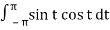 = ½ sin2 t
  = 0 – 0 = 0
Thus, sin t and cos t are orthogonal functions in the vector space C [- ]
]
Symmetric matrix:
In linear algebra, a symmetric matrix is a square matrix that is equal to its transpose. Formally, because equal matrices have equal dimensions, only square matrices can be symmetric. The entries of a symmetric matrix are symmetric with respect to the main diagonal. So, if aᵢⱼ denotes the entry in the i-th row and j-th column then for all indices i and j. Every square diagonal matrix is symmetric, since all off-diagonal elements are zero.
Any square matrix is said to be symmetric matrix if its transpose equals to the matrix itself.
For example:
 &
& 
Example: check whether the following matrix A is symmetric or not?
A = 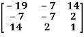
Sol. As we know that if the transpose of the given matrix is same as the matrix itself then the matrix is called symmetric matrix.
So that, first we will find its transpose,
Transpose of matrix A,

Here,
A = 
So that, the matrix A is symmetric.
Example: Show that any square matrix can be expressed as the sum of symmetric matrix and anti- symmetric matrix.
Sol. Suppose A is any square matrix
Then,
A = 
Now,
(A + A’)’ = A’ + A
A+A’ is a symmetric matrix.
Also,
(A - A’)’ = A’ – A
Here A’ – A is an anti – symmetric matrix
So that,
Square matrix = symmetric matrix + anti-symmetric matrix
Example: Let us test whether the given matrices are symmetric or not i.e., we check for,
A = 
(1) A = 
Now
 =
=
 A =
A = 
Hence the given matric symmetric
Example: let A be a real symmetric matrix whose diagonal entries are all positive real numbers.
Is this true for all of the diagonal entries of the inverse matrix A-1 are also positive? If so, prove it. Otherwise give a counter example
Solution: The statement is false, hence we give a counter example
Let us consider the following 2 2 matrix
A = 
The matrix A satisfies the required conditions, that is A is symmetric and its diagonal entries are positive.
The determinant det(A) = (1)(1)-(2)(2) = -3 and the inverse of A is given by
A-1=  =
= 
By the formula for the inverse matrix for 2 2 matrices.
This shows that the diagonal entries of the inverse matric A-1 are negative.
Skew-symmetric:
A skew-symmetric matrix is a square matrix that is equal to the negative of its own transpose. Anti-symmetric matrices are commonly called as skew-symmetric matrices.
In other words-
Skew-symmetric matrix-
A square matrix A is said to be skew symmetrix matrix if –
1. A’ = -A, [ A’ is the transpose of A]
2. All the main diagonal elements will always be zero.
For example-
A = 
This is skew symmetric matrix, because transpose of matrix A is equals to negative A.
Example: check whether the following matrix A is symmetric or not?
A = 
Sol. This is not a skew symmetric matrix, because the transpose of matrix A is not equals to -A.
-A = A’
Example: Let A and B be n n skew-matrices. Namely AT = -A and BT = -B
(a) Prove that A+B is skew-symmetric.
(b) Prove that cA is skew-symmetric for any scalar c.
(c) Let P be an m n matrix. Prove that PTAP is skew-symmetric.
Solution: (a) (A+B)T = AT + BT = (-A) +(-B) = -(A+B)
Hence A+B is skew symmetric.
(b) (cA)T = c.AT =c(-A) = -cA
Thus, cA is skew-symmetric.
(c)Let P be an m n matrix. Prove that PT AP is skew-symmetric.
Using the properties, we get,
(PT AP)T = PTAT(PT)T = PTATp
= PT (-A) P = - (PT AP)
Thus (PT AP) is skew-symmetric.
Key takeaways-
- Any square matrix is said to be symmetric matrix if its transpose equals to the matrix itself.
- Square matrix = symmetric matrix + anti-symmetric matrix
- A skew-symmetric matrix is a square matrix that is equal to the negative of its own transpose. Anti-symmetric matrices are commonly called as skew-symmetric matrices.
Quadratic forms & Nature of the Quadratic forms-
Quadratic form can be expressed as a product of matrices.
Q(x) = X’ AX,
Where,
X =  and A =
X’ is the transpose of X,
X’AX = [ x1 x2 x3] 
= [ a11x1 + a21x2 + a31x3 a12x1 + a22x2 + a32x3 a13x1 + a23x2 + a33x3]
= a11x12 + a21x1x2 + a31 x1x3 + a12x1x2 + a22x22 +a32x2x3 + a13x1x3 + a23x2x3 + a33x32
= a11x12 + a22x22+a33x32+(a12+a21)x1x2 + (a23+ a32)x2x+(a31+ a13)x1x3
Which is the quadratic form.
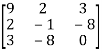
Example: find out the quadratic form of following matrix.
A = 
Solution: Quadratic form is,
X’ AX
= [x1 x2 x3] = [ x1 + 2x2 + 5x3, 2x1 + 3x3, 5x1 + 3x2 + 4x3]
= x12 + 2x1x2 + 5x3x1 + 2x1x2 + 3x2x3 + 5x1x3 + 3x2x3 + 4x32
= x12 + 4x32 + 4 x1x2 + 10x1x3 + 6 x2x3
Which is the quadratic form of a matrix.
Example: Find the real matrix of the following quadratic form:
Q(x1, x2, x3) = x2 + 4x22 + 6x32 + 2x1x2 + x2x3 + 3x1x3
Sol. Here we will compare the coefficients with the standard quadratic equation,
We get,
a11 = 1, a22 = 4, a33 = 6, a12 = 2, a21 = 0, a23 = 1, a32 = 0, a13 = 3, a31 = 0
Q(x1, x2, x3) = [x1 x2 x3] = [ x1 2x1+4x2 3x1 + x2+ 6x3]
= x12 + 2x1x2 + 4x22 + 3x1x3 + x2x3 + 6x32
Definition: Let V be a vector space over F. An inner product on V is a function that assigns, to every ordered pair of vectors x and y in V, a scalar in F, denoted  , such that for all x, y, and z in V and all c in F, the following hold:
(a) 
(b) 
(c) 
(d) 
Note that (c) reduces to =
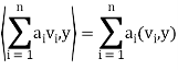
=  if F = R. Conditions (a) and (b) simply require that the inner product be linear in the first component.
It is easily shown that if  and
and  , then

Example: For x = ( ) and y = (
 ) in
) in  , define

The verification that  satisfies conditions (a) through (d) is easy. For example, if z = (
 ) we have for (a)

Thus, for x = (1+i, 4) and y = (2 − 3i,4 + 5i) in 
A vector space V over F endowed with a specific inner product is called an inner product space. If F = C, we call V a complex inner product It is clear that if V has an inner product  and W is a subspace of
V, then W is also an inner product space when the same function  is
is
Restricted to the vectors x, y ∈ W space, whereas if F = R, we call V a real inner product space.
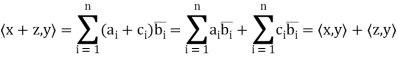
Theorem: Let V be an inner product space. Then for x, y, z ∈ V and c ∈ F, the following statements are true.
(a) 
(b) 
(c) 
(d) 
(e) If 
Norms:
Let V be an inner product space. For x ∈ V, we define the norm or length of x by ||x|| = 
Key takeaways:
Let V be a vector space over F. An inner product on V is a function that assigns, to every ordered pair of vectors x and y in V
Gram- Schmidt orthogonalization process
Suppose { } is a basis of an inner product space V. One can use this basis to construct an orthogonal basis {
 } of V as follows. Set


………………
……………….
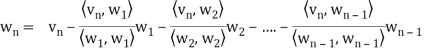
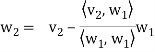
In other words, for k = 2, 3, . . . , n, we define

Where

Is the component of  .
.
Each  is orthogonal to the preceeding w’s. Thus,
 form an orthogonal basis for V as claimed. Normalizing each wi will then yield an orthonormal basis for V.
The above process is known as the Gram–Schmidt orthogonalization process.
Note-
- Each vector wk is a linear combination of
 and the preceding w’s. Hence, one can easily show, by induction, that each
  is a linear combination of
- Because taking multiples of vectors does not affect orthogonality, it may be simpler in hand calculations to clear fractions in any new
 , by multiplying
  by an appropriate scalar, before obtaining the next
  .
.
Theorem: Let  be any basis of an inner product space V. Then there exists an orthonormal basis
  of V such that the change-of-basis matrix from {
 to {
to { is triangular; that is, for k = 1; . . . ; n,
uk = ak1v1 + ak2v2 + . . . + akkvk
Theorem: Suppose S =  is an orthogonal basis for a subspace W of a vector space V. Then one may extend S to an orthogonal basis for V; that is, one may find vectors
  ,
, such that
  is an orthogonal basis for V.
Example: Apply the Gram–Schmidt orthogonalization process to find an orthogonal basis and then an orthonormal basis for the subspace U of  spanned by

Sol:
Step-1: First  =
= 
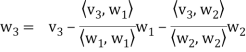
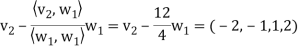
Step-2: Compute

Now set- 
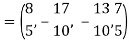
Step-3: Compute
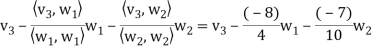

Clear fractions to obtain, 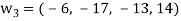
Thus,  ,
,  ,
,  form an orthogonal basis for U. Normalize these vectors to obtain an orthonormal basis
 of U. We have


So

Reduction of quadratic form to canonical form by orthogonal transformation
A real symmetric matrix ‘A’ can be reduced to a diagonal form M’AM = D ………(1)
Where M is the normalized orthogonal modal matrix of A and D is its spectoral matrix.
Suppose the orthogonal transformation is-
X =MY
Q = X’AX = (MY)’ A (MY) = (Y’M’) A (MY) = Y’(M’AM) Y
= Y’DY
= Y’ diagonal ( )Y
)Y
= [y1 y2 … yn]
= [ λ1 y1 λ2y2 …. λnyn] 
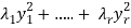
= λ1y12 + λ2y22 + …. + λnyn2
Which is called canonical form.
Step by step method for Reduction of quadratic form to canonical form by orthogonal transformation –
1. Construct the symmetric matrix A associated to the given quadratic form  .
.
2. Now for the characteristic equation-
|A -  | = 0
| = 0
Then find the eigen values of A. Let  be the positive eigen values arranged in decreasing oeder , that means ,
3. An orthogonal canonical reduction of the given quadratic form is-

4. Obtain an order system of n orthonormal vector  consisting of eigen vectors corresponding to the eigen values
  .
.
5. Construct the orthogonal matrix P whose columns are the eigen vectors 
6. The recurred change of basis is given by X = PY
7. The new basis { } is called the canonical basis and its elements are principal axes of the given quadratic form.
Example: Find the orthogonal canonical form of the quadratic form.
5
Sol. The matrix form of this quadratic equation can be written as,
A = 
We can find the eigen values of A as –
|A -  | = 0
| = 0
 = 0
= 0

Which gives,

The required orthogonal canonical reduction will be,
8 .
.
Least Squares Approximation
Suppose a survey conducted by taking two measurements such as  at times
  respectively.
For example the surveyor wants to measure the birth rate at various times during a given period.
Suppose the collected data set  is plotted as points in the plane.
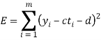
From this plot, the surveyer finds that there exists a linear relationship between the two variables, y and t, say- y = ct + d, and would like to find the constants c and d so that the line y = ct + d represents the best possible fit to the data collected. One such estimate of fit is to calculate the error E that represents the sum of the squares of the vertical distances from the points to the line; that is,

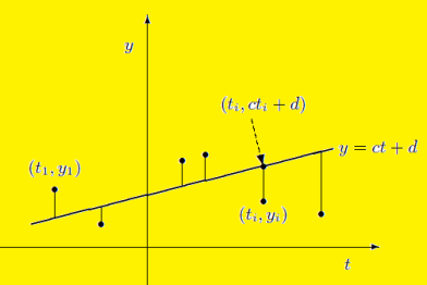
Thus we reduce this problem to finding the constants c and d that minimize
E.( the line y = ct + d is called the least squares line)
If we suppose,
A = 
Then it follows-

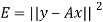
We develop a general method for finding an explicit vector  that minimizes E; that is, given an m × n matrix A, we find
  such that
  for all vectors
  .
.
This method not only allows us to find the linear function that best fits the data, but also, for any positive integer n, the best fit using a polynomial of degree at most n.
For  , let
, let  denote the standard inner product of x and y in
  . Recall that if x and y are regarded as column vectors, then

First lemma: Suppose  then
then

Second lemma: Suppose  , then rank(
Note- If A is an m × n matrix such that rank(A) = n, then  is invertible.
Theorem: let  then there exists
  such that
 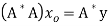 and
and  for all
  .
.
Furthermore, if rank (A) = n, then 
Example: Suppose the data collected by surveyor is (1, 2), (2, 3), (3, 5) and (4, 7), then
A = 
Hence
A *A = 
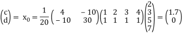
Thus
Therefore,

It follows that the line y = 1.7t is the least squares line. The error E is computed as 
Two square matrix  and A of same order n are said to be similar if and only if
 for some non singular matrix P.
Such transformation of the matrix A into  with the help of non singular matrix P is known as similarity transformation.
Similar matrices have the same Eigen values.
If X is an Eigen vector of matrix A then  is Eigen vector of the matrix
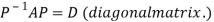
Reduction to Diagonal Form:
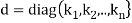
Let A be a square matrix of order n has n linearly independent Eigen vectors Which form the matrix P such that

Where P is called the modal matrix and D is known as spectral matrix.
Procedure: let A be a square matrix of order 3.
Let three Eigen vectors of A are  Corresponding to Eigen values
Let 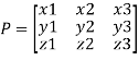
 {by characteristics equation of A}
Or 
Or 
Note: The method of diagonalization is helpful in calculating power of a matrix.
 .Then for an integer n we have
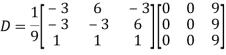
Example: Diagonalise the matrix 
Let A= 
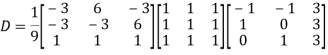
The three Eigen vectors obtained are (-1,1,0), (-1,0,1) and (3,3,3) corresponding to Eigen values  .
.
Then  and
and 
Also we know that 


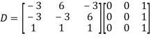
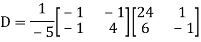
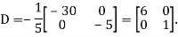
Example: Diagonalise the matrix
Let A =
The Eigen vectors are (4,1),(1,-1) corresponding to Eigen values  .
.
Then  and also
Also we know that 


Diagonalization of Linear Operators:
Consider a linear operator T: V  V. Then T is said to be diagonalizable if it can be represented by a diagonal matrix D. Thus, T is diagonalizable if and only if there exists a basis S = {
 } of V for which


………………
……………….

In such a case, T is represented by the diagonal matrix

Relative to the basis S.
References:
- E. Kreyszig, “Advanced Engineering Mathematics”, John Wiley & Sons, 2006.
- P. G. Hoel, S. C. Port And C. J. Stone, “Introduction To Probability Theory”, Universal Book Stall, 2003.
- S. Ross, “A First Course in Probability”, Pearson Education India, 2002.
- W. Feller, “An Introduction To Probability Theory and Its Applications”, Vol. 1, Wiley, 1968.
- N.P. Bali and M. Goyal, “A Text Book of Engineering Mathematics”, Laxmi Publications, 2010.
- B.S. Grewal, “Higher Engineering Mathematics”, Khanna Publishers, 2000.
Unit - 8
Inner product and Orthogonality
The definition of a vector space V involves an arbitrary field K. Here we first restrict K to be the real field R, in which case V is called a real vector space; in the last sections of this chapter, we extend our results to the case where K is the complex field C, in which case V is called a complex vector space. Also, we adopt the previous notation that
u; v;w are vectors in V
a; b; c; k are scalars in K
Furthermore, the vector spaces V in this chapter have finite dimension unless otherwise stated or implied.
Recall that the concepts of ‘‘length’’ and ‘‘orthogonality’’ did not appear in the investigation of arbitrary vector spaces V (although they did appear in Section 1.4 on the spaces Rn and Cn). Here we place an additional structure on a vector space V to obtain an inner product space, and in this context these concepts are defined.
Inner Product Spaces:
Def: Let V be a real vector space. Suppose to each pair of vectors u, v  V there is assigned a real number, denoted by <u, v>. This function is called a (real) inner product on V if it satisfies the following axioms:
(Linear Property): <au1 + bu2, v> = a <u1, v> + b <u2, v>
(Symmetric Property): <u, v> = <v, u>
(Positive Definite Property): <u, u>  and <u, u> = 0 if and only if u = 0.
The vector space V with an inner product is called a inner product space.
Note- an inner product of linear combinations of vectors is equal to a linear combination of the inner products of the vectors.
Norm of a Vector
By the third axiom of an inner product, <u, v> is nonnegative for any vector u. Thus, its positive square root exists. We use the notation
This nonnegative number is called the norm or length of u. The relation ||u||2 = <u, u> will be used frequently.
If ||u|| = 1 or, equivalently, if <u, u> = 1, then u is called a unit vector and it is said to be normalized. Every nonzero vector v in V can be multiplied by the reciprocal of its length to obtain the unit vector

Which is a positive multiple of v. This process is called normalizing v.
Orthogonality:
Let V be an inner product space. The vectors u, v  V are said to be orthogonal and u is said to be orthogonal to v if
<u, v> = 0
The relation is clearly symmetric—if u is orthogonal to v, then <v, u> = 0, and so v is orthogonal to u. We note that 0  V is orthogonal to every v
  V, because
Conversely, if u is orthogonal to every v 2 V, then <u, u> = 0 and hence u = 0 by third axiom: Observe that u and v are orthogonal if and only if cos y = 0, where y is the angle between u and v. Also, this is true if and only if u and v are ‘‘perpendicular’’—that is, y =  2 (or y = 90degree).
Example: Consider the vectors
u = (1, 1, 1), v = (1, 2, -3), w = (1, -4, 3) in R3.
Then
<u, v> =1+2 – 3 = 0, <u, w> = 1 – 4+3 = 0, <v, w> = 1 – 8 – 9 = - 16
Thus, u is orthogonal to v and w, but v and w are not orthogonal.
Example: Consider the functions sin t and cos t in the vector space C = [- ] of continuous functions on the closed interval [-
 ]. Then
< sin t, cos t> =  = ½ sin2 t
  = 0 – 0 = 0
Thus, sin t and cos t are orthogonal functions in the vector space C [- ]
]
Symmetric matrix:
In linear algebra, a symmetric matrix is a square matrix that is equal to its transpose. Formally, because equal matrices have equal dimensions, only square matrices can be symmetric. The entries of a symmetric matrix are symmetric with respect to the main diagonal. So, if aᵢⱼ denotes the entry in the i-th row and j-th column then for all indices i and j. Every square diagonal matrix is symmetric, since all off-diagonal elements are zero.
Any square matrix is said to be symmetric matrix if its transpose equals to the matrix itself.
For example:
 &
& 
Example: check whether the following matrix A is symmetric or not?
A = 
Sol. As we know that if the transpose of the given matrix is same as the matrix itself then the matrix is called symmetric matrix.
So that, first we will find its transpose,
Transpose of matrix A,

Here,
A = 
So that, the matrix A is symmetric.
Example: Show that any square matrix can be expressed as the sum of symmetric matrix and anti- symmetric matrix.
Sol. Suppose A is any square matrix
Then,
A = 
Now,
(A + A’)’ = A’ + A
A+A’ is a symmetric matrix.
Also,
(A - A’)’ = A’ – A
Here A’ – A is an anti – symmetric matrix
So that,
Square matrix = symmetric matrix + anti-symmetric matrix
Example: Let us test whether the given matrices are symmetric or not i.e., we check for,
A = 
(1) A = 
Now
 =
=
 A =
A = 
Hence the given matric symmetric
Example: let A be a real symmetric matrix whose diagonal entries are all positive real numbers.
Is this true for all of the diagonal entries of the inverse matrix A-1 are also positive? If so, prove it. Otherwise give a counter example
Solution: The statement is false, hence we give a counter example
Let us consider the following 2 2 matrix
A = 
The matrix A satisfies the required conditions, that is A is symmetric and its diagonal entries are positive.
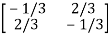
The determinant det(A) = (1)(1)-(2)(2) = -3 and the inverse of A is given by
A-1=  =
= 
By the formula for the inverse matrix for 2 2 matrices.
This shows that the diagonal entries of the inverse matric A-1 are negative.
Skew-symmetric:
A skew-symmetric matrix is a square matrix that is equal to the negative of its own transpose. Anti-symmetric matrices are commonly called as skew-symmetric matrices.
In other words-
Skew-symmetric matrix-
A square matrix A is said to be skew symmetrix matrix if –
1. A’ = -A, [ A’ is the transpose of A]
2. All the main diagonal elements will always be zero.
For example-
A = 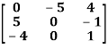
This is skew symmetric matrix, because transpose of matrix A is equals to negative A.
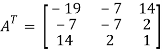
Example: check whether the following matrix A is symmetric or not?
A = 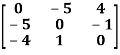
Sol. This is not a skew symmetric matrix, because the transpose of matrix A is not equals to -A.
-A = A’
Example: Let A and B be n n skew-matrices. Namely AT = -A and BT = -B
(a) Prove that A+B is skew-symmetric.
(b) Prove that cA is skew-symmetric for any scalar c.
(c) Let P be an m n matrix. Prove that PTAP is skew-symmetric.
Solution: (a) (A+B)T = AT + BT = (-A) +(-B) = -(A+B)
Hence A+B is skew symmetric.
(b) (cA)T = c.AT =c(-A) = -cA
Thus, cA is skew-symmetric.
(c)Let P be an m n matrix. Prove that PT AP is skew-symmetric.
Using the properties, we get,
(PT AP)T = PTAT(PT)T = PTATp
= PT (-A) P = - (PT AP)
Thus (PT AP) is skew-symmetric.
Key takeaways-
- Any square matrix is said to be symmetric matrix if its transpose equals to the matrix itself.
- Square matrix = symmetric matrix + anti-symmetric matrix
- A skew-symmetric matrix is a square matrix that is equal to the negative of its own transpose. Anti-symmetric matrices are commonly called as skew-symmetric matrices.
Quadratic forms & Nature of the Quadratic forms-
Quadratic form can be expressed as a product of matrices.
Q(x) = X’ AX,
Where,
X =  and A =
X’ is the transpose of X,
X’AX = [ x1 x2 x3] 
= [ a11x1 + a21x2 + a31x3 a12x1 + a22x2 + a32x3 a13x1 + a23x2 + a33x3]
= a11x12 + a21x1x2 + a31 x1x3 + a12x1x2 + a22x22 +a32x2x3 + a13x1x3 + a23x2x3 + a33x32
= a11x12 + a22x22+a33x32+(a12+a21)x1x2 + (a23+ a32)x2x+(a31+ a13)x1x3
Which is the quadratic form.
Example: find out the quadratic form of following matrix.
A = 
Solution: Quadratic form is,
X’ AX
= [x1 x2 x3] = [ x1 + 2x2 + 5x3, 2x1 + 3x3, 5x1 + 3x2 + 4x3]
= x12 + 2x1x2 + 5x3x1 + 2x1x2 + 3x2x3 + 5x1x3 + 3x2x3 + 4x32
= x12 + 4x32 + 4 x1x2 + 10x1x3 + 6 x2x3
Which is the quadratic form of a matrix.
Example: Find the real matrix of the following quadratic form:
Q(x1, x2, x3) = x2 + 4x22 + 6x32 + 2x1x2 + x2x3 + 3x1x3
Sol. Here we will compare the coefficients with the standard quadratic equation,
We get,
a11 = 1, a22 = 4, a33 = 6, a12 = 2, a21 = 0, a23 = 1, a32 = 0, a13 = 3, a31 = 0
Q(x1, x2, x3) = [x1 x2 x3] = [ x1 2x1+4x2 3x1 + x2+ 6x3]
= x12 + 2x1x2 + 4x22 + 3x1x3 + x2x3 + 6x32
Definition: Let V be a vector space over F. An inner product on V is a function that assigns, to every ordered pair of vectors x and y in V, a scalar in F, denoted  , such that for all x, y, and z in V and all c in F, the following hold:
(a) 
(b) 
(c) 
(d) 
Note that (c) reduces to =
=  if F = R. Conditions (a) and (b) simply require that the inner product be linear in the first component.
It is easily shown that if  and
and  , then

Example: For x = ( ) and y = (
 ) in
) in  , define

The verification that  satisfies conditions (a) through (d) is easy. For example, if z = (
 ) we have for (a)

Thus, for x = (1+i, 4) and y = (2 − 3i,4 + 5i) in 
A vector space V over F endowed with a specific inner product is called an inner product space. If F = C, we call V a complex inner product It is clear that if V has an inner product  and W is a subspace of
V, then W is also an inner product space when the same function  is
is
Restricted to the vectors x, y ∈ W space, whereas if F = R, we call V a real inner product space.
Theorem: Let V be an inner product space. Then for x, y, z ∈ V and c ∈ F, the following statements are true.
(a) 
(b) 
(c) 
(d) 
(e) If 
Norms:
Let V be an inner product space. For x ∈ V, we define the norm or length of x by ||x|| = 
Key takeaways:
Let V be a vector space over F. An inner product on V is a function that assigns, to every ordered pair of vectors x and y in V
Gram- Schmidt orthogonalization process
Suppose { } is a basis of an inner product space V. One can use this basis to construct an orthogonal basis {
 } of V as follows. Set


………………
……………….

In other words, for k = 2, 3, . . . , n, we define

Where

Is the component of  .
.
Each  is orthogonal to the preceeding w’s. Thus,
 form an orthogonal basis for V as claimed. Normalizing each wi will then yield an orthonormal basis for V.
The above process is known as the Gram–Schmidt orthogonalization process.
Note-
- Each vector wk is a linear combination of
 and the preceding w’s. Hence, one can easily show, by induction, that each
  is a linear combination of
- Because taking multiples of vectors does not affect orthogonality, it may be simpler in hand calculations to clear fractions in any new
 , by multiplying
  by an appropriate scalar, before obtaining the next
  .
.
Theorem: Let  be any basis of an inner product space V. Then there exists an orthonormal basis
  of V such that the change-of-basis matrix from {
 to {
to { is triangular; that is, for k = 1; . . . ; n,
uk = ak1v1 + ak2v2 + . . . + akkvk
Theorem: Suppose S =  is an orthogonal basis for a subspace W of a vector space V. Then one may extend S to an orthogonal basis for V; that is, one may find vectors
  ,
, such that
  is an orthogonal basis for V.
Example: Apply the Gram–Schmidt orthogonalization process to find an orthogonal basis and then an orthonormal basis for the subspace U of  spanned by

Sol:
Step-1: First  =
= 
Step-2: Compute

Now set- 
Step-3: Compute


Clear fractions to obtain, 
Thus,  ,
,  ,
,  form an orthogonal basis for U. Normalize these vectors to obtain an orthonormal basis
 of U. We have


So

Reduction of quadratic form to canonical form by orthogonal transformation
A real symmetric matrix ‘A’ can be reduced to a diagonal form M’AM = D ………(1)
Where M is the normalized orthogonal modal matrix of A and D is its spectoral matrix.
Suppose the orthogonal transformation is-
X =MY
Q = X’AX = (MY)’ A (MY) = (Y’M’) A (MY) = Y’(M’AM) Y
= Y’DY
= Y’ diagonal ( )Y
)Y
= [y1 y2 … yn]
= [ λ1 y1 λ2y2 …. λnyn] 
= λ1y12 + λ2y22 + …. + λnyn2
Which is called canonical form.
Step by step method for Reduction of quadratic form to canonical form by orthogonal transformation –
1. Construct the symmetric matrix A associated to the given quadratic form  .
.
2. Now for the characteristic equation-
|A -  | = 0
| = 0
Then find the eigen values of A. Let  be the positive eigen values arranged in decreasing oeder , that means ,
3. An orthogonal canonical reduction of the given quadratic form is-

4. Obtain an order system of n orthonormal vector  consisting of eigen vectors corresponding to the eigen values
  .
.
5. Construct the orthogonal matrix P whose columns are the eigen vectors 
6. The recurred change of basis is given by X = PY
7. The new basis { } is called the canonical basis and its elements are principal axes of the given quadratic form.
Example: Find the orthogonal canonical form of the quadratic form.
5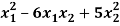
Sol. The matrix form of this quadratic equation can be written as,
A = 
We can find the eigen values of A as –
|A -  | = 0
| = 0
 = 0
= 0
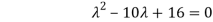
Which gives,

The required orthogonal canonical reduction will be,
8 .
.
Least Squares Approximation
Suppose a survey conducted by taking two measurements such as  at times
  respectively.
For example the surveyor wants to measure the birth rate at various times during a given period.
Suppose the collected data set 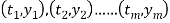 is plotted as points in the plane.
From this plot, the surveyer finds that there exists a linear relationship between the two variables, y and t, say- y = ct + d, and would like to find the constants c and d so that the line y = ct + d represents the best possible fit to the data collected. One such estimate of fit is to calculate the error E that represents the sum of the squares of the vertical distances from the points to the line; that is,


Thus we reduce this problem to finding the constants c and d that minimize
E.( the line y = ct + d is called the least squares line)
If we suppose,
A = 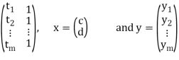
Then it follows-

We develop a general method for finding an explicit vector  that minimizes E; that is, given an m × n matrix A, we find
  such that
 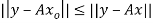 for all vectors
  .
.
This method not only allows us to find the linear function that best fits the data, but also, for any positive integer n, the best fit using a polynomial of degree at most n.
For  , let
, let  denote the standard inner product of x and y in
  . Recall that if x and y are regarded as column vectors, then

First lemma: Suppose  then
then

Second lemma: Suppose  , then rank(
Note- If A is an m × n matrix such that rank(A) = n, then  is invertible.
Theorem: let  then there exists
  such that
  and
and 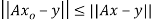 for all
  .
.
Furthermore, if rank (A) = n, then 
Example: Suppose the data collected by surveyor is (1, 2), (2, 3), (3, 5) and (4, 7), then
A = 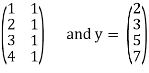
Hence
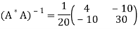
A *A = 
Thus

Therefore,
It follows that the line y = 1.7t is the least squares line. The error E is computed as 
Two square matrix  and A of same order n are said to be similar if and only if
 for some non singular matrix P.
Such transformation of the matrix A into  with the help of non singular matrix P is known as similarity transformation.
Similar matrices have the same Eigen values.
If X is an Eigen vector of matrix A then  is Eigen vector of the matrix
Reduction to Diagonal Form:
Let A be a square matrix of order n has n linearly independent Eigen vectors Which form the matrix P such that
Where P is called the modal matrix and D is known as spectral matrix.
Procedure: let A be a square matrix of order 3.
Let three Eigen vectors of A are  Corresponding to Eigen values
Let 
 {by characteristics equation of A}
Or 
Or 
Note: The method of diagonalization is helpful in calculating power of a matrix.
 .Then for an integer n we have
Example: Diagonalise the matrix 
Let A= 
The three Eigen vectors obtained are (-1,1,0), (-1,0,1) and (3,3,3) corresponding to Eigen values  .
.
Then  and
and 
Also we know that 


Example: Diagonalise the matrix
Let A =
The Eigen vectors are (4,1),(1,-1) corresponding to Eigen values  .
.
Then  and also
Also we know that 

Diagonalization of Linear Operators:
Consider a linear operator T: V  V. Then T is said to be diagonalizable if it can be represented by a diagonal matrix D. Thus, T is diagonalizable if and only if there exists a basis S = {
 } of V for which


………………
……………….

In such a case, T is represented by the diagonal matrix
Relative to the basis S.
References:
- E. Kreyszig, “Advanced Engineering Mathematics”, John Wiley & Sons, 2006.
- P. G. Hoel, S. C. Port And C. J. Stone, “Introduction To Probability Theory”, Universal Book Stall, 2003.
- S. Ross, “A First Course in Probability”, Pearson Education India, 2002.
- W. Feller, “An Introduction To Probability Theory and Its Applications”, Vol. 1, Wiley, 1968.
- N.P. Bali and M. Goyal, “A Text Book of Engineering Mathematics”, Laxmi Publications, 2010.
- B.S. Grewal, “Higher Engineering Mathematics”, Khanna Publishers, 2000.
Unit - 8
Inner product and Orthogonality
Unit - 8
Inner product and Orthogonality
Unit - 8
Inner product and Orthogonality
Unit - 8
Inner product and Orthogonality
Unit - 8
Inner product and Orthogonality
Unit - 8
Inner product and Orthogonality
The definition of a vector space V involves an arbitrary field K. Here we first restrict K to be the real field R, in which case V is called a real vector space; in the last sections of this chapter, we extend our results to the case where K is the complex field C, in which case V is called a complex vector space. Also, we adopt the previous notation that
u; v;w are vectors in V
a; b; c; k are scalars in K
Furthermore, the vector spaces V in this chapter have finite dimension unless otherwise stated or implied.
Recall that the concepts of ‘‘length’’ and ‘‘orthogonality’’ did not appear in the investigation of arbitrary vector spaces V (although they did appear in Section 1.4 on the spaces Rn and Cn). Here we place an additional structure on a vector space V to obtain an inner product space, and in this context these concepts are defined.
Inner Product Spaces:
Def: Let V be a real vector space. Suppose to each pair of vectors u, v  V there is assigned a real number, denoted by <u, v>. This function is called a (real) inner product on V if it satisfies the following axioms:
(Linear Property): <au1 + bu2, v> = a <u1, v> + b <u2, v>
(Symmetric Property): <u, v> = <v, u>
(Positive Definite Property): <u, u>  and <u, u> = 0 if and only if u = 0.
The vector space V with an inner product is called a inner product space.
Note- an inner product of linear combinations of vectors is equal to a linear combination of the inner products of the vectors.
Norm of a Vector
By the third axiom of an inner product, <u, v> is nonnegative for any vector u. Thus, its positive square root exists. We use the notation

This nonnegative number is called the norm or length of u. The relation ||u||2 = <u, u> will be used frequently.
If ||u|| = 1 or, equivalently, if <u, u> = 1, then u is called a unit vector and it is said to be normalized. Every nonzero vector v in V can be multiplied by the reciprocal of its length to obtain the unit vector

Which is a positive multiple of v. This process is called normalizing v.
Orthogonality:
Let V be an inner product space. The vectors u, v  V are said to be orthogonal and u is said to be orthogonal to v if
<u, v> = 0
The relation is clearly symmetric—if u is orthogonal to v, then <v, u> = 0, and so v is orthogonal to u. We note that 0  V is orthogonal to every v
  V, because
Conversely, if u is orthogonal to every v 2 V, then <u, u> = 0 and hence u = 0 by third axiom: Observe that u and v are orthogonal if and only if cos y = 0, where y is the angle between u and v. Also, this is true if and only if u and v are ‘‘perpendicular’’—that is, y =  2 (or y = 90degree).
Example: Consider the vectors
u = (1, 1, 1), v = (1, 2, -3), w = (1, -4, 3) in R3.
Then
<u, v> =1+2 – 3 = 0, <u, w> = 1 – 4+3 = 0, <v, w> = 1 – 8 – 9 = - 16
Thus, u is orthogonal to v and w, but v and w are not orthogonal.
Example: Consider the functions sin t and cos t in the vector space C = [- ] of continuous functions on the closed interval [-
 ]. Then
< sin t, cos t> =  = ½ sin2 t
  = 0 – 0 = 0
Thus, sin t and cos t are orthogonal functions in the vector space C [- ]
]
Symmetric matrix:
In linear algebra, a symmetric matrix is a square matrix that is equal to its transpose. Formally, because equal matrices have equal dimensions, only square matrices can be symmetric. The entries of a symmetric matrix are symmetric with respect to the main diagonal. So, if aᵢⱼ denotes the entry in the i-th row and j-th column then for all indices i and j. Every square diagonal matrix is symmetric, since all off-diagonal elements are zero.
Any square matrix is said to be symmetric matrix if its transpose equals to the matrix itself.
For example:
 &
& 
Example: check whether the following matrix A is symmetric or not?
A = 
Sol. As we know that if the transpose of the given matrix is same as the matrix itself then the matrix is called symmetric matrix.
So that, first we will find its transpose,
Transpose of matrix A,
Here,
A = 
So that, the matrix A is symmetric.
Example: Show that any square matrix can be expressed as the sum of symmetric matrix and anti- symmetric matrix.
Sol. Suppose A is any square matrix
Then,
A = 
Now,
(A + A’)’ = A’ + A
A+A’ is a symmetric matrix.
Also,
(A - A’)’ = A’ – A
Here A’ – A is an anti – symmetric matrix
So that,
Square matrix = symmetric matrix + anti-symmetric matrix
Example: Let us test whether the given matrices are symmetric or not i.e., we check for,
A = 
(1) A = 
Now
 =
=
 A =
A = 
Hence the given matric symmetric
Example: let A be a real symmetric matrix whose diagonal entries are all positive real numbers.
Is this true for all of the diagonal entries of the inverse matrix A-1 are also positive? If so, prove it. Otherwise give a counter example
Solution: The statement is false, hence we give a counter example
Let us consider the following 2 2 matrix
A = 
The matrix A satisfies the required conditions, that is A is symmetric and its diagonal entries are positive.
The determinant det(A) = (1)(1)-(2)(2) = -3 and the inverse of A is given by
A-1=  =
= 
By the formula for the inverse matrix for 2 2 matrices.
This shows that the diagonal entries of the inverse matric A-1 are negative.
Skew-symmetric:
A skew-symmetric matrix is a square matrix that is equal to the negative of its own transpose. Anti-symmetric matrices are commonly called as skew-symmetric matrices.
In other words-
Skew-symmetric matrix-
A square matrix A is said to be skew symmetrix matrix if –
1. A’ = -A, [ A’ is the transpose of A]
2. All the main diagonal elements will always be zero.
For example-
A = 
This is skew symmetric matrix, because transpose of matrix A is equals to negative A.
Example: check whether the following matrix A is symmetric or not?
A = 
Sol. This is not a skew symmetric matrix, because the transpose of matrix A is not equals to -A.
-A = A’
Example: Let A and B be n n skew-matrices. Namely AT = -A and BT = -B
(a) Prove that A+B is skew-symmetric.
(b) Prove that cA is skew-symmetric for any scalar c.
(c) Let P be an m n matrix. Prove that PTAP is skew-symmetric.
Solution: (a) (A+B)T = AT + BT = (-A) +(-B) = -(A+B)
Hence A+B is skew symmetric.
(b) (cA)T = c.AT =c(-A) = -cA
Thus, cA is skew-symmetric.
(c)Let P be an m n matrix. Prove that PT AP is skew-symmetric.
Using the properties, we get,
(PT AP)T = PTAT(PT)T = PTATp
= PT (-A) P = - (PT AP)
Thus (PT AP) is skew-symmetric.
Key takeaways-
- Any square matrix is said to be symmetric matrix if its transpose equals to the matrix itself.
- Square matrix = symmetric matrix + anti-symmetric matrix
- A skew-symmetric matrix is a square matrix that is equal to the negative of its own transpose. Anti-symmetric matrices are commonly called as skew-symmetric matrices.
Quadratic forms & Nature of the Quadratic forms-
Quadratic form can be expressed as a product of matrices.
Q(x) = X’ AX,
Where,
X =  and A =
X’ is the transpose of X,
X’AX = [ x1 x2 x3] 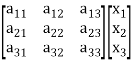
= [ a11x1 + a21x2 + a31x3 a12x1 + a22x2 + a32x3 a13x1 + a23x2 + a33x3]
= a11x12 + a21x1x2 + a31 x1x3 + a12x1x2 + a22x22 +a32x2x3 + a13x1x3 + a23x2x3 + a33x32
= a11x12 + a22x22+a33x32+(a12+a21)x1x2 + (a23+ a32)x2x+(a31+ a13)x1x3
Which is the quadratic form.
Example: find out the quadratic form of following matrix.
A = 
Solution: Quadratic form is,
X’ AX
= [x1 x2 x3] = [ x1 + 2x2 + 5x3, 2x1 + 3x3, 5x1 + 3x2 + 4x3]
= x12 + 2x1x2 + 5x3x1 + 2x1x2 + 3x2x3 + 5x1x3 + 3x2x3 + 4x32
= x12 + 4x32 + 4 x1x2 + 10x1x3 + 6 x2x3
Which is the quadratic form of a matrix.
Example: Find the real matrix of the following quadratic form:
Q(x1, x2, x3) = x2 + 4x22 + 6x32 + 2x1x2 + x2x3 + 3x1x3
Sol. Here we will compare the coefficients with the standard quadratic equation,
We get,
a11 = 1, a22 = 4, a33 = 6, a12 = 2, a21 = 0, a23 = 1, a32 = 0, a13 = 3, a31 = 0
Q(x1, x2, x3) = [x1 x2 x3] = [ x1 2x1+4x2 3x1 + x2+ 6x3]
= x12 + 2x1x2 + 4x22 + 3x1x3 + x2x3 + 6x32
Definition: Let V be a vector space over F. An inner product on V is a function that assigns, to every ordered pair of vectors x and y in V, a scalar in F, denoted  , such that for all x, y, and z in V and all c in F, the following hold:
(a) 
(b) 
(c) 
(d) 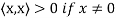
Note that (c) reduces to =
=  if F = R. Conditions (a) and (b) simply require that the inner product be linear in the first component.
It is easily shown that if  and
and  , then
Example: For x = ( ) and y = (
 ) in
) in  , define

The verification that  satisfies conditions (a) through (d) is easy. For example, if z = (
 ) we have for (a)
Thus, for x = (1+i, 4) and y = (2 − 3i,4 + 5i) in 
A vector space V over F endowed with a specific inner product is called an inner product space. If F = C, we call V a complex inner product It is clear that if V has an inner product  and W is a subspace of
V, then W is also an inner product space when the same function  is
is
Restricted to the vectors x, y ∈ W space, whereas if F = R, we call V a real inner product space.
Theorem: Let V be an inner product space. Then for x, y, z ∈ V and c ∈ F, the following statements are true.
(a) 
(b) 
(c) 
(d) 
(e) If 
Norms:
Let V be an inner product space. For x ∈ V, we define the norm or length of x by ||x|| = 
Key takeaways:
Let V be a vector space over F. An inner product on V is a function that assigns, to every ordered pair of vectors x and y in V
Gram- Schmidt orthogonalization process
Suppose { } is a basis of an inner product space V. One can use this basis to construct an orthogonal basis {
 } of V as follows. Set


………………
……………….

In other words, for k = 2, 3, . . . , n, we define

Where

Is the component of  .
.
Each  is orthogonal to the preceeding w’s. Thus,
 form an orthogonal basis for V as claimed. Normalizing each wi will then yield an orthonormal basis for V.
The above process is known as the Gram–Schmidt orthogonalization process.
Note-
- Each vector wk is a linear combination of
 and the preceding w’s. Hence, one can easily show, by induction, that each
  is a linear combination of
- Because taking multiples of vectors does not affect orthogonality, it may be simpler in hand calculations to clear fractions in any new
 , by multiplying
  by an appropriate scalar, before obtaining the next
  .
.
Theorem: Let  be any basis of an inner product space V. Then there exists an orthonormal basis
  of V such that the change-of-basis matrix from {
 to {
to { is triangular; that is, for k = 1; . . . ; n,
uk = ak1v1 + ak2v2 + . . . + akkvk
Theorem: Suppose S =  is an orthogonal basis for a subspace W of a vector space V. Then one may extend S to an orthogonal basis for V; that is, one may find vectors
  ,
, such that
  is an orthogonal basis for V.
Example: Apply the Gram–Schmidt orthogonalization process to find an orthogonal basis and then an orthonormal basis for the subspace U of  spanned by

Sol:
Step-1: First  =
= 
Step-2: Compute
Now set- 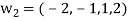
Step-3: Compute

Clear fractions to obtain, 
Thus,  ,
,  ,
,  form an orthogonal basis for U. Normalize these vectors to obtain an orthonormal basis
 of U. We have


So

Reduction of quadratic form to canonical form by orthogonal transformation
A real symmetric matrix ‘A’ can be reduced to a diagonal form M’AM = D ………(1)
Where M is the normalized orthogonal modal matrix of A and D is its spectoral matrix.
Suppose the orthogonal transformation is-
X =MY
Q = X’AX = (MY)’ A (MY) = (Y’M’) A (MY) = Y’(M’AM) Y
= Y’DY
= Y’ diagonal ( )Y
)Y
= [y1 y2 … yn]
= [ λ1 y1 λ2y2 …. λnyn] 
= λ1y12 + λ2y22 + …. + λnyn2
Which is called canonical form.
Step by step method for Reduction of quadratic form to canonical form by orthogonal transformation –
1. Construct the symmetric matrix A associated to the given quadratic form  .
.
2. Now for the characteristic equation-
|A -  | = 0
| = 0
Then find the eigen values of A. Let  be the positive eigen values arranged in decreasing oeder , that means ,
3. An orthogonal canonical reduction of the given quadratic form is-
4. Obtain an order system of n orthonormal vector  consisting of eigen vectors corresponding to the eigen values
  .
.
5. Construct the orthogonal matrix P whose columns are the eigen vectors 
6. The recurred change of basis is given by X = PY
7. The new basis { } is called the canonical basis and its elements are principal axes of the given quadratic form.
Example: Find the orthogonal canonical form of the quadratic form.
5
Sol. The matrix form of this quadratic equation can be written as,
A = 
We can find the eigen values of A as –
|A -  | = 0
| = 0
 = 0
= 0

Which gives,

The required orthogonal canonical reduction will be,
8 .
.
Least Squares Approximation
Suppose a survey conducted by taking two measurements such as  at times
  respectively.
For example the surveyor wants to measure the birth rate at various times during a given period.
Suppose the collected data set  is plotted as points in the plane.
From this plot, the surveyer finds that there exists a linear relationship between the two variables, y and t, say- y = ct + d, and would like to find the constants c and d so that the line y = ct + d represents the best possible fit to the data collected. One such estimate of fit is to calculate the error E that represents the sum of the squares of the vertical distances from the points to the line; that is,

Thus we reduce this problem to finding the constants c and d that minimize
E.( the line y = ct + d is called the least squares line)
If we suppose,
A = 
Then it follows-
We develop a general method for finding an explicit vector  that minimizes E; that is, given an m × n matrix A, we find
  such that
  for all vectors
  .
.
This method not only allows us to find the linear function that best fits the data, but also, for any positive integer n, the best fit using a polynomial of degree at most n.
For  , let
, let  denote the standard inner product of x and y in
  . Recall that if x and y are regarded as column vectors, then

First lemma: Suppose  then
then
Second lemma: Suppose  , then rank(
Note- If A is an m × n matrix such that rank(A) = n, then  is invertible.
Theorem: let  then there exists
  such that
  and
and  for all
  .
.
Furthermore, if rank (A) = n, then 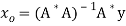
Example: Suppose the data collected by surveyor is (1, 2), (2, 3), (3, 5) and (4, 7), then
A = 
Hence
A *A = 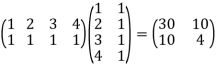
Thus

Therefore,

It follows that the line y = 1.7t is the least squares line. The error E is computed as 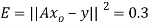
Two square matrix  and A of same order n are said to be similar if and only if
 for some non singular matrix P.
Such transformation of the matrix A into  with the help of non singular matrix P is known as similarity transformation.
Similar matrices have the same Eigen values.
If X is an Eigen vector of matrix A then  is Eigen vector of the matrix
Reduction to Diagonal Form:
Let A be a square matrix of order n has n linearly independent Eigen vectors Which form the matrix P such that

Where P is called the modal matrix and D is known as spectral matrix.
Procedure: let A be a square matrix of order 3.
Let three Eigen vectors of A are  Corresponding to Eigen values
Let 
 {by characteristics equation of A}
Or 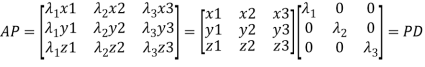
Or 
Note: The method of diagonalization is helpful in calculating power of a matrix.
 .Then for an integer n we have
Example: Diagonalise the matrix 
Let A= 
The three Eigen vectors obtained are (-1,1,0), (-1,0,1) and (3,3,3) corresponding to Eigen values  .
.
Then 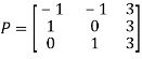 and
and 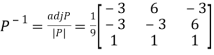
Also we know that 


Example: Diagonalise the matrix
Let A =
The Eigen vectors are (4,1),(1,-1) corresponding to Eigen values  .
.
Then  and also
Also we know that 


Diagonalization of Linear Operators:
Consider a linear operator T: V  V. Then T is said to be diagonalizable if it can be represented by a diagonal matrix D. Thus, T is diagonalizable if and only if there exists a basis S = {
 } of V for which


………………
……………….

In such a case, T is represented by the diagonal matrix

Relative to the basis S.
References:
- E. Kreyszig, “Advanced Engineering Mathematics”, John Wiley & Sons, 2006.
- P. G. Hoel, S. C. Port And C. J. Stone, “Introduction To Probability Theory”, Universal Book Stall, 2003.
- S. Ross, “A First Course in Probability”, Pearson Education India, 2002.
- W. Feller, “An Introduction To Probability Theory and Its Applications”, Vol. 1, Wiley, 1968.
- N.P. Bali and M. Goyal, “A Text Book of Engineering Mathematics”, Laxmi Publications, 2010.
- B.S. Grewal, “Higher Engineering Mathematics”, Khanna Publishers, 2000.


