Module 1
Calculus
i) f(x) is continuous in the closed [a, b]
Ii) f(x) is differentiable in (a, b) &
Iii) f(a) = f(b)
Then there exist at least one value ‘c’ in (a, b) such that f’(c) = 0.
Exercise 1
Verify Rolle’s theorem for the function f(x) = x2 for 
Solution:
Here f(x) = x2; 
i) Since f(x) is algebraic polynomial which is continuous in [-1, 1]
Ii) Consider f(x) = x2
Diff. w.r.t. x we get
f'(x) = 2x
Clearly f’(x) exist in (-1, 1) and does not becomes infinite.
Iii) Clearly
f(-1) = (-1)2 = 1
f(1) = (1)2 = 1
 f(-1) = f(1).
Hence by Rolle’s theorem, there exist  such that
f’(c) = 0
i.e. 2c = 0
 c = 0
c = 0
Thus  such that
f'(c) = 0
Hence Rolle’s Theorem is verified.
Exercise 2
Verify Rolle’s Theorem for the function f(x) = ex(sin x – cos x) in 
Solution:
Here f(x) = ex(sin x – cos x); 
i) Clearly ex is an exponential function continuous for every  also sin x and cos x are Trigonometric functions Hence (sin x – cos x) is continuous in
  and Hence ex(sin x – cos x) is continuous in
  .
.
Ii) Consider
f(x) = ex(sin x – cos x)
Diff. w.r.t. x we get
f’(x) = ex(cos x + sin x) + ex(sin x + cos x)
= ex[2sin x]
Clearly f’(x) is exist for each  & f’(x) is not infinite.
Hence f(x) is differentiable in  .
.
Iii) Consider


Also,


Thus 
Hence all the conditions of Rolle’s theorem are satisfied, so there exist  such, that

i.e. 
i.e. sin c = 0


But

Hence Rolle’s theorem is verified.
Exercise 3
Verify whether Rolle’s theorem is applicable or not for

Solution:
Here f(x) = x2; 
i) Clearly x2 is an algebraic polynomial hence it is continuous in [2, 3]
Ii) Consider


Clearly f’(x) is exist for each 
Iii) Consider


Thus  .
.
Thus all conditions of Rolle’s theorem are not satisfied Hence Rolle’s theorem is not applicable for f(x) = x2 in [2, 3]
Exercise 4
- Show that between any two real root of equation
 , is at least one real root of
  .
. - Discuss the applicability of Rolle’s theorem for the function

Lagrange’s Mean value Theorem:-
Statement:- If
i) f(x) is continuous in [a, b]
Ii) f(x) is differentiable in (a, b) then there exist at least one value  such that

Exercise 5
Verify the Lagrange’s mean value theorem for

Solution:
Here 
i) Clearly f(x) = log x is logarithmic function. Hence it is continuous in [1, e]
Ii) Consider f(x) = log x.
Diff. w.r.t. x we get,

Clearly f’(x) is exist for each value of  & is finite.
Hence all conditions of LMVT are satisfied Hence at least 
Such that

i.e. 
i.e. 
i.e. 
i.e. 
Since e = 2.7183

Clearly c = 1.7183 
Hence LMVT is verified.
Exercise 6
Verify mean value theorem for f(x) = tan-1x in [0, 1]
Solution:
Here  ;
; 
i) Clearly  is an inverse trigonometric function and hence it is continuous in [0, 1]
Ii) Consider 
Diff. w.r.t. x we get,

Clearly f’(x) is continuous and differentiable in (0, 1) & is finite
Hence all conditions of LMVT are satisfied, Thus there exist 
Such that

i.e. 

i.e. 
i.e. 

i.e. 


Clearly 
Hence LMVT is verified.
Meaning of sign of Derivative:
Let f(x) satisfied LMVT in [a, b]
Let x1 and x2 be any two points laying (a, b) such that x1 < x2
Hence by LMVT,  such that
i.e.  … (1)
… (1)
Cast I:
If 
 then
then 
i.e. 
 is constant function
Case II:
If 
 then from equation (1)

i.e. 
 means x2 - x1 > 0 and
Thus for x2 > x1

Thus f(x) is increasing function is (a, b)
Case III:
If 

Then from equation (1)

i.e. 

Since  and
and  then
then 
 hence f(x) is strictly decreasing function.
Exercise 7
Prove that

And hence show that

Solution:
Let  ;
; 
i) Clearly  is an logarithmic function and hence it is continuous also
Ii) Consider 

Diff. w.r.t. x we get,

Clearly f’(x) exist and finite in (a, b) Hence f(x) is continuous and differentiable in (a, b). Hence by LMVT 
Such that

i.e. 
i.e. 
Since
a < c < b


i.e. 
i.e. 
i.e. 
i.e. 
Hence the result
Now put a = 5, b = 6 we get


Hence the result
Exercise 8
Prove that  ,
,  use mean value theorem to prove that,

Hence show that

Solution:
Let f(x) = sin-1x; 
i) Clearly f(x) is inverse trigonometric function and hence it is continuous in [a, b]
Ii) Consider f(x) = sin-1x
Diff. w.r.t. x we get,

Clearly f’(x) is finite and exist for  . Hence by LMVT,
  such that

i.e. 
Since a < c < b


i.e. 
i.e. 
i.e. 
i.e. 
Hence the result
Put  we get

i.e. 
i.e. 
i.e. 
i.e. 
Hence the result
Statement:-
If f(x) and g(x) are any two functions such that
a) f(x) and g(x) are continuous in (a, b)
b) both f(x) and g(x) are derivable in (a, b)
c) 
Then for any value of  ,
,  at least
  such that

Exercise
Verify Cauchy mean value theorems for  &
&  in
in 
Solution:
Let  &
&  ;
; 
i) Clearly f(x) and g(x) both are trigonometric functions. Hence continuous in 
Ii) Since  &
& 
Diff. w.r.t. x we get,
 &
& 
Clearly both f’(x) and g’(x) exist & finite in  . Hence f(x) and g(x) is derivable in
  and
and
Iii) 

Hence by Cauchy mean value theorem, there exist at least  such that

i.e. 

i.e. 1 = cot c

i.e. 
Clearly 
Hence Cauchy mean value theorem is verified.
Exercise
Considering the functions ex and e-x, show that c is arithmetic mean of a & b.
Solution:
i) Clearly f(x) and g(x) are exponential functions Hence they are continuous in [a, b].
Ii) Consider  &
& 
Diff. w.r.t. x we get
 and
and 
Clearly f(x) and g(x) are derivable in (a, b)
 By Cauchy’s mean value theorem
  such that

i.e. 
i.e. 
i.e. 
i.e. 
i.e. 
i.e. 

Thus 
i.e. c is arithmetic mean of a & b.
Hence the result
Exercise
Show that 
Prove that if 
 and Hence show that

Verify Cauchy’s mean value theorem for the function x2 and x4 in [a, b] where a, b > 0
If for  then prove that,

[Hint: ,
,  ]
]
Expansions of functions
In this topic we learn two important series expansions namely
i) Maclaurin’s series
Ii) Taylors Series
Maclaurin’s Series Expansions
Statement:-
Maclaurin’s series of f(x) at x = 0 is given by,

Expansion of some standard functions
i) f(x) = ex then

Proof:-
Here


 By Maclaurin’s series we get,

i.e. 
Note that
- Replace x by –x we get

2. f(x) = sin x then

Proof:
Let (x) = sin x
Then by Maclaurin’s series,
 … (1)
… (1)
Since


 By equation (i) we get,


3.  Then
Then

Proof:
Let f(x) = cos x
Then by Maclaurin’s series,
 … (1)
… (1)
Since


 From Equation (1)


4.  then
then

Proof:
Here f(x) = tan x
 By Maclaurin’s expansion,
 … (1)
… (1)
Since


 …..
…..
 By equation (1)


5.  Then
Then

Proof:-
Here f(x) = sin hx.
 By Maclaurin’s expansion,
 (1)
(1)


 By equation (1) we get,


6.  . Then

Proof:-
Here f(x) = cos hx
 By Maclaurin’s expansion
 (1)
(1)


 By equation (1)


7. f(x) = tan hx

Proof:
Here f(x) = tan hx
 By Maclaurin’s series expansion,
 … (1)
… (1)


 By equation (1)


8.  then
then

Proof:-
Here f(x) = log (1 + x)
 By Maclaurin’s series expansion,
 … (1)
… (1)


 By equation (1)


9. 
In above result we replace x by -x
Then


10. Expansion of tan h-1x
We know that


Thus

11. Expansion of (1 + x)m
Proof:-
Let f(x) = (1 + x)m
 By Maclaurin’s series.
 … (1)
… (1)


 By equation (1) we get,


Note that in above expansion if we replace m = -1 then we get,


Now replace x by -x in above we get,

Expand by, Maclaurin’s theorem

Solution:
Here f(x) = log (1 + sin x)
 By Maclaurin’s Theorem,
 … (1)
… (1)


 ……..
……..
 equation (1) becomes,


Expand by Maclaurin’s theorem
Log sec x
Solution:
Let f(x) = log sec x
 By Maclaurin’s Expansion’s,
 (1)
(1)


 By equation (1)


Prove that 
Solution:
Here f(x) = x cosec x
= 
Now we know that


Expand  upto x6
Solution:
Here 


Now we know that
 … (1)
… (1)
 … (2)
… (2)
Adding (1) and (2) we get

Show that 
Solution:
Here 


Thus

a) The expansion of f(x+h) in ascending power of x is

b) The expansion of f(x+h) in ascending power of h is

c) The expansion of f(x) in ascending powers of (x-a) is,

Using the above series expansion we get series expansion of f(x+h) or f(x).
Expansion of functions using standard expansions
Expand  in power of (x – 3)
Solution:
Let 
Here a = 3
Now by Taylor’s series expansion,
 … (1)
… (1)


 equation (1) becomes.


Using Taylors series method expand
 in powers of (x + 2)
Solution:
Here 
a = -2
 By Taylors series,
 … (1)
… (1)
Since


 ,
,  , …..
, …..
Thus equation (1) becomes


Expand  in ascending powers of x.
Solution:
Here

i.e. 

Here h = -2
 By Taylors series,
 … (1)
… (1)


 equation (1) becomes,


Thus


Expand  in powers of x using Taylor’s theorem,
Solution:
Here


i.e. 
Here
h = 2
 By Taylors series
 … (1)
… (1)


 By equation (1)


Exercise
a) Expand  in powers of (x – 2)
b) Expand  in powers of (x + 2)
c) Expand  in powers of (x – 1)
d) Using Taylors series, express  in ascending powers of x.
e) Expand  in powers of x, using Taylor’s theorem.
Partial Differentiation of composite function
a) Let  and
and  , then z becomes a function of
  , In this case z is called composite function of
  .
.
i.e.

b) Let  possess continuous partial derivatives and let
  possess continuous partial derivatives, then z is called composite function of x and y.
i.e.

& 
Continuing in this way, …..
Ex. If  Then prove that

Ex. If  then prove that

Where  is function of x, y, z.
Ex. If  where
where  ,
,
 then show that,
i) 
Ii) 
Notations of partial derivatives of variable to be treated as a constant
Let
 and
and 
i.e.

Then  means partial derivative of u w.r.t. x treating y const.
To find  from given reactions we first express x in terms of u & v.
i.e.  & then diff. x w.r.t. u treating v constant.
To find  express v as a function of y and u i.e.
  then diff. v w.r.t. y treating u as a const.
Ex. If  ,
,  then find the value of
 .
.
Ex. If  ,
,  then prove that

Ex.1: Evaluate 0∞ x3/2 e -x dx
Solution: 0∞ x3/2 e -x dx = 0∞ x 5/2-1 e -x dx
= γ(5/2)
= γ(3/2+ 1)
= 3/2 γ(3/2 )
= 3/2 . ½ γ(½ )
= 3/2 . ½ .π
= ¾ π
Ex. 2: Find γ(-½)
Solution: (-½) + 1 = ½
γ(-1/2) = γ(-½ + 1) / (-½)
= - 2 γ(1/2 )
= - 2 π
Ex. 3. Show that 

Solution : =
= 

= 


= 


 ) .......................
= 

= 


Ex. 4: Evaluate 
 dx.
dx.
Solution : Let 

 dx
dx
X | 0 |  |
t | 0 |  |
Put  or
or  ;dx =2t dt .
 dt
dt
 dt
dt


Ex. 5: Evaluate  dx.
dx.
Solution : Let 
 dx.
dx.
x | 0 |  |
t | 0 |  |
Put  or
or  ; 4x dx = dt
 dx
dx


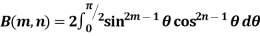
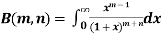
Definition : Beta function
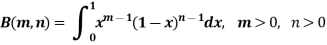
|
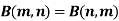
Properties of Beta function : |
2.  |
3.  |
4. 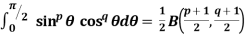 |
Example(1): Evaluate I = 
Solution:
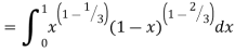

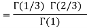

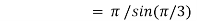
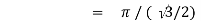
= 2 π/3
Example(2): Evaluate: I = 02 x2 / (2 – x ) . Dx
Solution:
Letting x = 2y, we get
I = (8/2) 01 y 2 (1 – y ) -1/2dy
= (8/2) . B(3 , 1/2 )
= 642 /15
BETA FUNCTION MORE PROBLEMS
Relation between Beta and Gamma functions :
  | ||||||
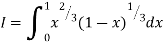
Example(1): Evaluate: I = 0a x4 (a2 – x2 ) . Dx Solution: Letting x2 = a2 y , we get I = (a6 / 2) 01 y 3/2 (1 – y )1/2dy = (a6 / 2) . B(5/2 , 3/2 ) = a6 /3 2 Example(2): Evaluate: I = 02 x (8 – x3 ) . Dx Solution: Let x3 = 8y I = (8/3) 01 y-1/3 (1 – y ) 1/3 . Dy
= (8/3) B(2/3 , 4/3 ) = 16 π / ( 9 3 ) Example(3): Prove that  Solution : Let   Put            Example(4): Evaluate  Solution :Let  Put      When    
Also             
Example(5): Show that  Solution :  =             Exercise : - Q. Show that 1.   |


Let  be a function of x, y, z which to be discussed for stationary value.
Let  be a relation in x, y, z
 for stationary values we have,

i.e.  … (1)
… (1)
Also from  we have
 … (2)
… (2)
Let ‘ ’ be undetermined multiplier then multiplying equation (2) by
  and adding in equation (1) we get,

 … (3)
… (3)
 … (4)
… (4)
 … (5)
… (5)
Solving equation (3), (4) (5) & we get values of x, y, z and  .
.
- Decampere a positive number ‘a’ in to three parts, so their product is maximum
Solution:
Let x, y, z be the three parts of ‘a’ then we get.
 … (1)
… (1)
Here we have to maximize the product
i.e. 
 By Lagrange’s undetermined multiplier, we get,

 … (2)
… (2)
 … (3)
… (3)
 … (4)
… (4)
i.e.
 … (2)’
 … (3)’
 … (4)
… (4)


And 


From (1)


Thus  .
.
Hence their maximum product is  .
.
2. Find the point on plane  nearest to the point (1, 1, 1) using Lagrange’s method of multipliers.
Solution:
Let  be the point on sphere
  which is nearest to the point
  . Then shortest distance.


 Let
Let 
Under the condition  … (1)
… (1)
 By method of Lagrange’s undetermined multipliers we have

 … (2)
… (2)

 … (3)
… (3)
i.e.  &
&

 … (4)
… (4)
From (2) we get 
From (3) we get 
From (4) we get 
 Equation (1) becomes

i.e. 


y = 2

If  where x + y + z = 1.
Prove that the stationary value of u is given by,

References
1. G.B. Thomas and R.L. Finney, Calculus and Analytic geometry, 9th Edition,Pearson, Reprint, 2002.
2. Erwin kreyszig, Advanced Engineering Mathematics, 9th Edition, John Wiley & Sons, 2006.
3. Veerarajan T., Engineering Mathematics for first year, Tata McGraw-Hill, New Delhi, 2008.
4. Ramana B.V., Higher Engineering Mathematics, Tata McGraw Hill New Delhi, 11thReprint, 2010.
5. D. Poole, Linear Algebra: A Modern Introduction, 2nd Edition, Brooks/Cole, 2005.
6. N.P. Bali and Manish Goyal, A text book of Engineering Mathematics, Laxmi Publications, Reprint, 2008.
7. B.S. Grewal, Higher Engineering Mathematics, Khanna Publishers, 36th Edition, 2010.


