Module 2
Calculus
When we apply limits in indefinite integrals are called definite integrals.
If an expression is written as  , here ‘b’ is called upper limit and ‘a’ is called lower limit.
If f is an increasing or decreasing function on interval [a , b], then


Where 
Properties-
1. The definite integral applies only if a<b, but it would be appropriate to include the case a = b and a>b as well, in that case-
If a = b, then

And if a>b, then
2. Integral of a constant function-
3. Constant multiple property-
4. Interval union property-
If a < c < b, then
5. Inequality-
If c and d are constants such that  for all x in [a , b], then
c(b – a)
Note- if a function f:[a , b]→R is continuous, then the function ‘f’ is always Integrable.
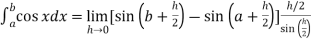
Example-1: Evaluate .
.
Sol. Here we notice that f:x→cos x is a decreasing function on [a , b],
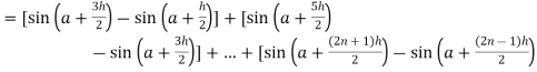
Therefore by the definition of the definite integrals-

Then

Now,


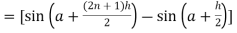
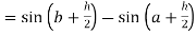
Here 
Thus
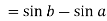
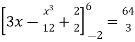
Example-2: Evaluate 
Sol. Here  is an increasing function on [1 , 2]
So that,
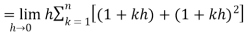
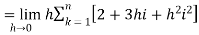
 …. (1)
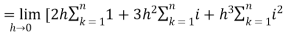
We know that-


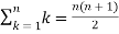
And

Then equation (1) becomes-

Note- we can find the definite integral directly as-

Example-3: Evaluate- 


Sol. 
A function,
Is called gamma function of n , which can be written as,
Some important results-


Ex.1: Evaluate 0∞ x3/2 e -x dx
Solution: 0∞ x3/2 e -x dx = 0∞ x 5/2-1 e -x dx
= γ (5/2)
= γ (3/2+ 1)
= 3/2 γ (3/2 )
= 3/2. ½ γ (½ )
= 3/2 .½.π
= ¾ π
Ex. 2: Find γ(-½)
Solution: (-½) + 1 = ½
γ(-1/2) = γ(-½ + 1) / (-½)
= - 2 γ (1/2 )
= - 2 π
Ex. 3. Show that 

Solution: =
= 

= 


= 


 ) .......................
= 

= 


Ex. 4: Evaluate 
 dx.
dx.
Solution: Let 

 dx
dx
X | 0 |  |
t | 0 |  |
Put  or
or ;dx =2t dt .
 dt
dt
 dt
dt


Ex. 5: Evaluate  dx.
dx.
Solution : Let 
 dx.
dx.
x | 0 |  |
t | 0 |  |
Put  or
or  ; 4x dx = dt
 dx
dx


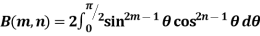
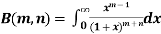
Definition : Beta function
|
Properties of Beta function : |
2.  |
3.  |
4. 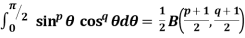 |
Example(1): Evaluate I = 
Solution:
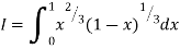
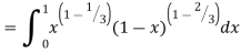

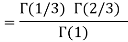

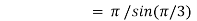
= 2 π/3
Example(2): Evaluate: I = 02 x2 / (2 – x ) . Dx
Solution:
Letting x = 2y, we get
I = (8/2) 01 y 2 (1 – y ) -1/2dy
= (8/2) . B(3 , 1/2 )
= 642 /15
BETA FUNCTION MORE PROBLEMS
Relation between Beta and Gamma functions :
  | ||||||
Example(1): Evaluate: I = 0a x4 (a2 – x2 ) . Dx Solution: Letting x2 = a2 y , we get I = (a6 / 2) 01 y 3/2 (1 – y )1/2dy = (a6 / 2) . B(5/2 , 3/2 ) = a6 /3 2 Example(2): Evaluate: I = 02 x (8 – x3 ) . Dx Solution: Let x3 = 8y I = (8/3) 01 y-1/3 (1 – y ) 1/3 . Dy
= (8/3) B(2/3 , 4/3 ) = 16 π / ( 9 3 ) Example(3): Prove that  Solution : Let   Put            Example(4): Evaluate  Solution :Let  Put      When    
Also             
Example(5): Show that  Solution :  =             |


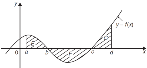
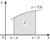
Area under and between the curves-
Total shaded area will be as follows of the given figure( by using definite integrals)-
Total shaded area = 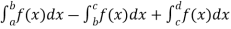
Example-1: Determine the area enclosed by the curves-
Sol. We know that the curves are equal at the points of interaction, thus equating the values of y of each curve-

Which gives-

By factorization,
Which means,
x = 2 and x = -3
By determining the intersection points the range the values of x has been found-
x | -3 | -2 | -1 | 0 | 1 | 2 |
 | 10 | 5 | 2 | 1 | 2 | 5 |
And
x | -3 | 0 | 2 |
y = 7 - x | 10 | 7 | 5 |
We get the following figure by using above two tables-
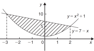
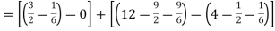
Area of shaded region = 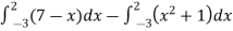
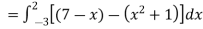
= 
= ( 12 – 2 – 8/3 ) – (-18 – 9/2 + 9)
= 
= 125/6 square unit
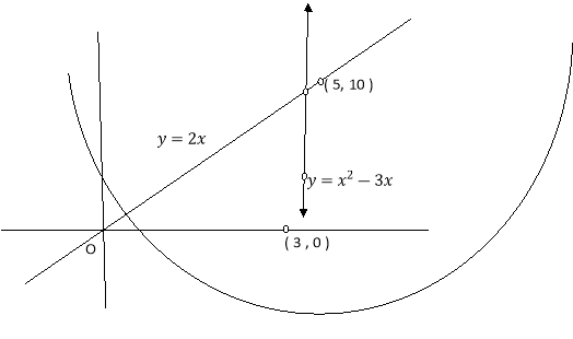
Example-2: Determine the area bounded by three straight lines y = 4 – x, y = 3x and 3y = x
Sol. We get the following figure by using the equations of three straight lines-
y = 4 – x, y = 3x and 3y = x
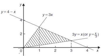
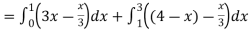
Area of shaded region-
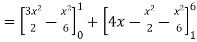
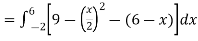
Example-3: Find the area enclosed by the two functions-
 and g(x) = 6 – x
Sol. We get the following figure by using these two equations 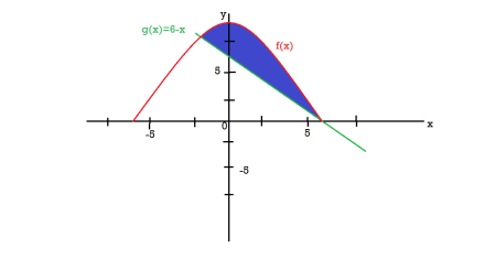
To find the intersection points of two functions f(x) and g(x)-
f(x) = g(x)
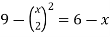

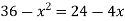
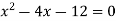
On factorizing, we get-
x = 6, -2
Now

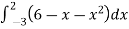
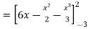
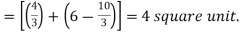
Then, area under the curve-
A = 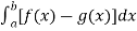
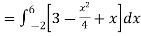
Therefore the area under the curve is 64/3 square unit.
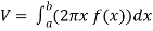
The volume of revolution (V) is obtained by rotating area A through one revolution about the x-axis is given by-

Suppose the curve x = f(y) is rotated  about y-axis between the limits y = c and y = d, then the volume generated V, is given by-

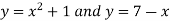
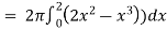
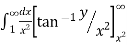
Example-1: Find the area enclosed by the curves 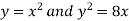 and if the area is rotated
  about the x-axis then determine the volume of the solid of revolution.
Sol. We know that, at the point of intersection the coordinates of the curve are equal. So that first we will find the point of intersection-


We get,
x = 0 and x = 2
The curve of the given equations will look like as follows-
Then,
The area of the shaded region will be-
A = 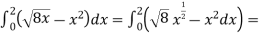
So that the area will be 8/3 square unit.
The volume will be
= (volume produced by revolving  – (volume produced by revolving
= 
Method of cylindrical shells-
Let f(x) be a continuous and positive function. Define R as the region bounded above by the graph f(x), below by the x-axis, on the left by the line x = a and on the right x = b, then the volume of the solid of revolution formed by revolving R around the y-axis is given by
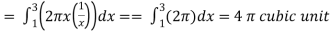
Example-2: Find the volume of the solid of revolution formed by revolving R around y-axis of the function f(x) = 1/x over the interval [1 , 3].
Sol. The graph of the function f(x) = 1/x will look like-
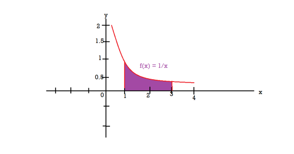
The volume of the solid of revolution generated by revolving R(violet region) about the y-axis over the interval [1 , 3]
Then the volume of the solid will be-
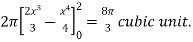
Example-3: Find the volume of the solid of revolution formed by revolving R around y-axis of the function f(x) = 2x - x² over the interval [0 , 2].
Sol. The graph of the function f(x) = 2x - x² will be-
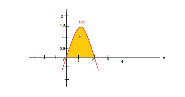
The volume of the solid is given by-

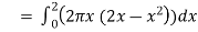
= 
Double integral –
Before studying about multiple integrals , first let’s go through the definition of definition of definite integrals for function of single variable.
As we know, the integral

Where is belongs to the limit a ≤ x ≤ b
This integral can be written as follows-

Now suppose we have a function f(x , y) of two variables x and y in two dimensional finite region R in xy-plane.
Then the double integration over region R can be evaluated by two successive integration

Evaluation of double integrals-
If A is described as 
Then,
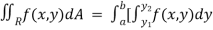 ]dx
]dx
Let do some examples to understand more about double integration-
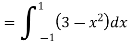
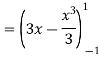
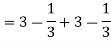
Example-1: Evaluate  , where dA is the small area in xy-plane.
Sol. Let , I = 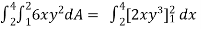
= 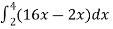
= 
= 
= 84 sq. Unit.
Which is the required area.
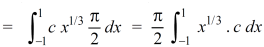
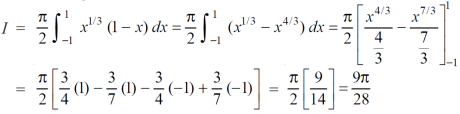
Example-2: Evaluate 
Sol. Let us suppose the integral is I,
I = 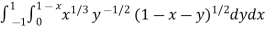
Put c = 1 – x in I, we get
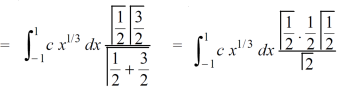
I = 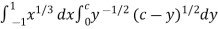
Suppose , y = ct
Then dy = c
Now we get,
I = 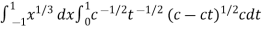
I = 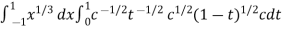
I = 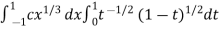
I = 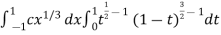
I = 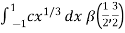
As we know that by beta function,
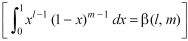
Which gives,
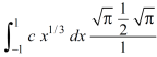
Now put the value of c, we get
Example-3: Evaluate the following double integral,
Sol. Let ,
I = 
On solving the integral, we get
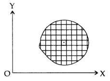
Double Integral over Rectangular and general regions
Consider a function f (x, y) defined in the finite region R of the x-y plane. Divide R into n elementary areas A1, A2,…,An. Let (xr, yr) be any point within the rth elementary are Ar
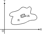
Fig. 6.1
f (x, y) dA = f (xr, yr) A
Evaluation of Double Integral when limits of Integration are given(Cartesian Form).
Ex. 1 : Evaluate  ey/x dy dx.
Soln. :
Given : I =  ey/x dy dx
Here limits of inner integral are functions of y therefore integrate w.r.t y,
I = 
 dx
dx
= 
= 
I = 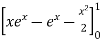
= =
 ey/x dy dx =
Ex. 2 : Evaluate x y
y (1 – x –y)
 dx dy.
Soln. :
Given : I = x y
y (1 – x –y)
 dx dy.
Here the limits of inner integration are functions of y therefore first integrate w.r.t y.
I = x dx
dx 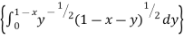
Put 1 – x = a (constant for inner integral)
I = x dx
dx 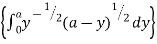
Put y = at dy = a dt
y | 0 | a |
t | 0 | 1 |
I = x dx
dx 
I = x dx
dx 
I = x a dx
a dx
I = x (1 – x) dx = (x
 – x4/3) dx
I = 
=
I = =
x y
y (1 – x –y)
 dx dy =
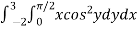
Ex. 3 : Evaluate 
Soln. :
Let, I = 
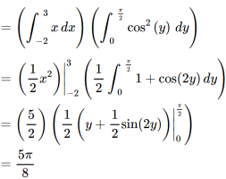
Here limits for both x and y are constants, the integral can be evaluated first w.r.t any of the variables x or y.
I = dy 
I = 
= 
= 
= 
=
= 
 =
=
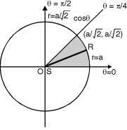
Ex. 4: Evaluate e–x2 (1 + y2) x dx dy.
Soln. :
Let I = e–x2 (1 + y2) x dy = dy e–x2 (1 + y2) x dy
= dy e– x2 (1 + y2)  dx
dx
= dy [∵ f (x) ef(x) dx = ef(x) ]
= (–1) dy (∵ e– = 0)
= = =
e–x2 (1 + y2) xdx dy =
NOTES:
Type II: Evaluation of Double Integral when region of Integration is provided (Cartesian form)
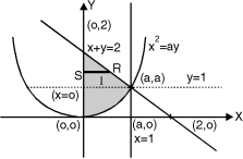
Ex.1: Evaluate y dx dy over the area bounded by x= 0 y =  and x + y = 2 in the first quadrant
Soln. :
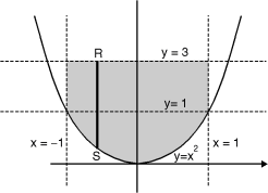
The area bounded by y = x2 (parabola) and x + y = 2 is as shown in Fig.6.2
The point of intersection of y = x2 and x + y = 2.
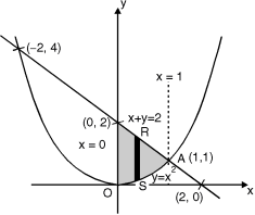
x + x2 = 2 x2 + x – 2 = 0
x = 1, – 2
At x = 1, y = 1 and at x = –2, y = 4
Fig. 6.2
(1, 1) is the point of intersection in Ist quadrant. Take a vertical strip SR, Along SR x constant and y varies from S to R i.e. y = x2 to y = 2 – x.
Now slide strip SR, keeping IIel to y-axis, therefore y constant and x varies from x = 0 to x = 1.
I = 
= 
= 
= (4 – 4x +  –
–  ) dx
) dx
= =
I = 16/15
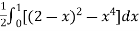
Ex. 2 : Evaluate  over x 1, y
Soln. :
 Let I =
  over x 1, y
The region bounded by x 1 and y 
Is as shown in Fig. 6.3.
Fig. 6.3
Take a vertical strip along strip x constant and y varies from y = 
To y = . Now slide strip throughout region keeping parallel to y-axis. Therefore y constant and x varies from x = 1 to x = .
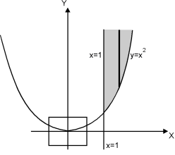
I = 
= 
=  [ ∵
[ ∵ dx = tan–1 (x/a)]
=  =
=
= – = (0 – 1)
I =
Ex. 3 : Evaluate ( +
+  ) dx dy through the area enclosed by the curves y = 4x, x + y = 3 and y =0, y = 2.
Soln. :
Let I = ( +
+  ) dx dy
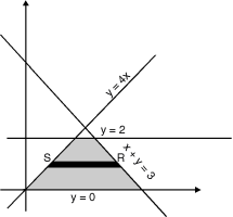 The area enclosed by the curves y = 4x, x + y =3, y = 0 and y = 2 is as shown in Fig. 6.4.
(find the point of intersection of x + y = 3 and y = 4x)
Fig. 6.4
Take a horizontal strip SR, along SR y constant and x varies from x = to x = 3 – y. Now slide strip keeping IIel to x axis therefore x constant and y varies from y = 0 to y = 2.
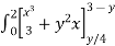
I = dy ( +
+  ) dx
) dx
= 
=  +
+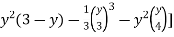 dy
dy
I = 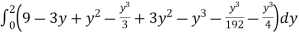
= 
= 
= + – 6 + 18
I =
Ex.1: Change the order of integration for the integral  and evaluate the same with reversed order of integration.
Sol:
Given, I =  …(1)
…(1)
 In the given integration, limits are
y =  , y = 2a – x and x = 0, x = a
The region bounded by x2 = ay, x + y = 2a Fig.6.5
And x = 0, x = a is as shown in Fig. 6.5
Here we have to change order of Integration. Given the strip is vertical.
Now take horizontal strip SR.
To take total region, Divide region into two parts by taking line y = a.
1 st Region:
Along strip, y constant and x varies from x = 0 to x = 2a – y. Slide strip IIel to x-axis therefore y varies from y = a to y = 2a.
I1 = dy xy dx …(2)
2nd Region:
Along strip, y constant and x varies from x = 0 to x= . Slide strip IIel to x-axis therefore x-varies from y = 0 to y = a.
I2 = dy xy dx …(3)
From Equation (1), (2) and (3),
 = dy xy dx + dy xy dx
= 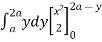 + y dy
= dy + (ay) dy = y (4a2 – 4ay + y2) dy + ay2 dy
= (4a2 y – 4ay2 + y3) dy + y2 dy
= 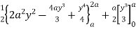
= 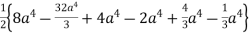 +
+ 
= a4
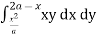
 Ex. 2 : Evaluate
I = 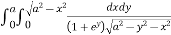
Soln. :
 Given : I =
  …(1)
…(1)
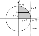
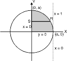
In the given integration, limits are
x = 0, x = a, y = 0, y = 
The bounded region is as shown in Fig. **.
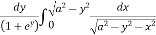
In the given, strip is vertical. Now take horizontal strip SR. Along strip y constant and x varies from x = 0 to
x =  . Slide strip IIel to X-axis therefore y varies from y = 0 to y = a.
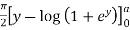
I = dy 
= 
Put a2 – y2 = b2
I = 

=  =
= 
=  dy =
dy =  dy
dy
= 
=
= 
=  [∵ a = a loge]
I = dy  =
= 
 Ex.3 : Express as single integral and evaluate dy dx + dy dx.
Soln. :
Given : I = dy dx + dy dx
I = I1 + I2
The limits of region of integration I1 are
x = – ; x = and y = 0, y = 1 and I2 are x = – 1,
x = 1 and y = 1, y = 3.
The region of integration are as shown in Fig. 6.7
To consider the complete region take a vertical strip SR along the strip y varies from y = x2 to
y = 3 and x varies from x = –1 to x = 1. Fig. 6.7
I = 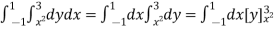

NOTES:
Evaluation of Double Integral by Changing Cartesian to Polar co-ordinates (when limits are given).
 Ex. 1 : Evaluate
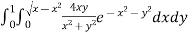
Soln. :
The region of integration bounded by
y = 0, y =  and x = 0, x = 1
y =  x2 + y2 = x
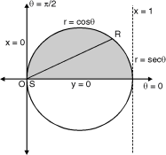
The region bounded by these is as shown in Fig. 6.8.
Convert the integration in polar co-ordinates by using x = r cos , y = r sin and dx dy = r dr d
x2 + y2 = x becomes r = cos
y = 0 becomes r sin = 0 = 0
x = 0 becomes r cos = 0 =
And x = 1 becomes r = sec Fig. 6.8
Take a radial strip SR with angular thickness , Along strip constant and r varies from r = 0 to r = cos . Turning strip throughout region therefore varies from = 0 to =
I =  r dr d
= 4 cos sin d r  dr
dr
= 4 cos sin d [– ]
]
= – 2 cos sin [ +1] d
+1] d
= – 2 [cos sin  – cos sin ] d
= –2  + 2 cos sin d
= – + 2
= + 1 =
 Ex. 2: Sketch the area of double integration and evaluate
 dxdy
dxdy
Soln. :
Let I =  dxdy
dxdy
The region of integration is bounded by the curves
x = y, x =  and y = 0, y = Fig. 6.9
i.e. x = y, x2 + y2 = a2 and y = 0, y =
The region bounded by these is as shown in Fig. 6.9.
The point of intersection of x = y and x2 + y2 = a2 is x =
Convert given integration in polar co-ordinates by using polar transformation x = r cos , y = r sin and dx dy = r dr d
x = y gives r cos = r sin tan = 1 =
x2 + y2 = a2 r2 = a2 r = a
y = 0 gives r sin = 0 = 0.
y = gives r sin = r = cosec
Take a radial strip SR, along SR constant and r varies from r = 0 to r = a. Turning this strip throughout region therefore varies from = 0 to =
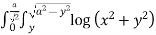
I = log r2 r dr d = 2 d r log r dr
I = 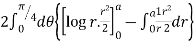
= 2 d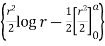
= 2 d
= 2  d
d
= 2  []
[]
I =  [/4] =
Evaluation of Double Integral when region of Integration is provided (Polar form)
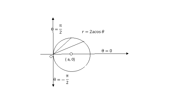
Ex. 1 : Evaluate r4 cos3 dr d over the interior of the circle r = 2a cos
Soln. :
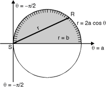 The region of the integration is as shown in Fig. 6.10.Take a radial strip SR, along strip constant and r varies from r = 0 to r = 2a cos. Now turning this strip throughout region therefore varies from = to =
I = r4 cos3 dr d
= cos3 d
=  cos3 cos5 d
=  cos8 d Fig. 6.10
= 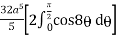
=  2
2
I = 
r4 cos3 dr d = 
Ex. 2 : Evaluate r sin dr d over the cardioid r = a (1 – cos ) above the initial line.
Soln. :
The cardioid r = a (1 – cos ) is as shown in Fig. 6.11. The region of the integration is above the initial line.
Take a radial strip SR, along strip constant and r Varies from r = 0 to r = a (1 – cos ).
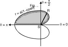 New turning the strip throughout region therefore varies from = 0 to = .
I = r sin dr d
= sin d
Fig.6.11
= sin [a2 (1 – cos )2]
= 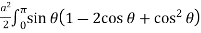
I =  (sin – 2 sin cos + sin
  ) d
) d
=  2 (sin – sin2 + sin
  ) d
) d
= 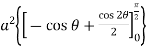 +
+
I = a2= a2
I = 
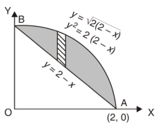
Area in Cartesian coordinates-
Example-1: Find the area enclosed by two curves using double integration.
y = 2 – x and y² = 2 (2 – x)
Sol. Let,
y = 2 – x ………………..(1)
And y² = 2 (2 – x) ………………..(2)
On solving eq. (1) and (2)
We get the intersection points (2,0) and (0,2) ,
We know that,
Area = 
Here we will find the area as below,
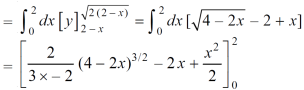
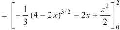
Area = 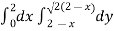
Which gives,
= ( - 4 + 4 /2 ) + 8 / 3 = 2 / 3.
Example-2: Find the area between the parabola y ² = 4ax and another parabola x² = 4ay.
Sol. Let,
y ² = 4ax ………………..(1)
And
x² = 4ay…………………..(2)
Then if we solve these equations, we get the values of points where these two curves intersect
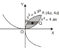
x varies from y²/4a to  and y varies from o to 4a,
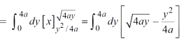
Now using the conceot of double integral,
Area = 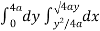
Area in polar coordinates-
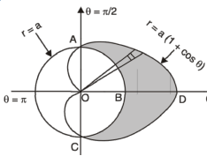
Example-3: Find the area lying inside the cardioid r = a(1+cosθ) and outside the circle r = a, by using double integration.
Sol. We have,
r = a(1+cosθ) …………………….(1)
And
r = a ……………………………….(2)
On solving these equations by eliminating r , we get
a(1+cosθ) = a
(1+cosθ) = 1
Cosθ = 0
Here a θ varies from – π/2 to π/2
Limit of r will be a and 1+cosθ)
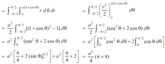
Which is the required area.
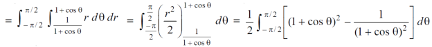
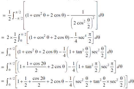
Example-4: Find the are lying inside a cardioid r = 1 + cos θ and outside the parabola r(1 + cos θ) = 1.
Sol. Let,
r = 1 + cos θ ……………………..(1)
r(1 + cos θ) = 1……………………..(2)
Solving these equations , we get
(1 + cos θ )( 1 + cos θ ) = 1
(1 + cos θ )² = 1
1 + cos θ = 1
Cos θ = 0
θ = ±π / 2
So that, limits of r are,
1 + cos θ and 1 / 1 + cos θ
The area can be founded as below,
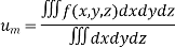
Volume by triple integral-
The volume of solid is given by
Volume =
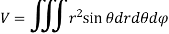
In Spherical polar system
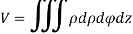
In cylindrical polar system
Ex.1: Find Volume of the tetrahedron bounded by the co-ordinates planes and the plane

Solution: Volume = ………. (1)
Put  ,
, 
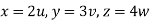
From equation (1) we have
V = 
=24
=24 (u+v+w=1) By Dirichlet’s theorem.
=24 
= =
= = 4
= 4
Volume =4
Ex.2: Find volume common to the cylinders ,
,  .
.
Solution: For given cylinders,
 ,
,  .
.
Z varies from
Z=- to z =
Y varies from
y= - to y =
x varies from x= -a to x = a
By symmetry,
Required volume= 8 (volume in the first octant)
=8 
=8
= 8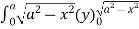 dx
dx
=8
=8
=8
Volume = 16
Ex.3: Evaluate
1.  Solution: -


Ex.4:


Ex.5:Evaluate 
Solution:- Put


NOTES:
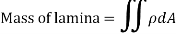
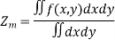
MASS OF A LAMINA :- If the surface density ρ of a plane lamina is a function of the position of a point of the lamina, then the mass of an elementary area dA is ρ dA and the total mass of the lamina is 
In Cartesian coordinates, if ρ = f(x, y) the mass of lamina, M=
In polar coordinates, if ρ = F(r, Ө) the mass of lamina, M=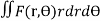
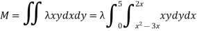
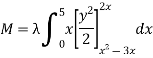
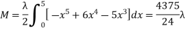
Ex.1: A lamina is bounded by the curves  and
and  . If the density at any point is
  then find mass of lamina.
Solution:
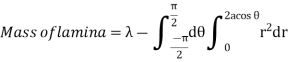
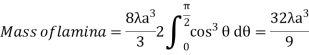
Ex.2:If the density at any point of a non-uniform circular lamina of radius’ a’ varies as its distance from a fixed point on the circumference of the circle then find the mass of lamina.
Solution:
Take the fixed point on the circumference of the circle as origin and diameter through it as x axis. The polar equation of circle 
And density .
.
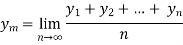
Mean Value:
The mean value of the ordinate y of a function  over the range
  to
to  is the limit of mean value of the equidistant ordinates
  as
as 

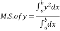
Mean Square values of function  over the range
  to
to  is defined as
Mean Square values of function 
Mean Square values of function 
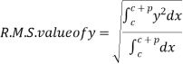
Root Mean Square Value: (R.M.S. Value):
If y is a periodic function of x of period p, the root mean square value of y is the square root of the mean value of  over the range
  to
to  , c is constant.
Ex. 1: Find mean value and R.M.S. Value of the ordinate of cycloid
 ,
,  over the range
  to
to  .
.
Sol Let P(x,y) be any point on the cycloid . Its ordinate is y.


= 
=
=
R.M.S.Value = 


Ex. 2: Find The Mean Value of  Over the positive octant of the
Ellipsoid 
Sol: M.V.=
Since 
Put 


M.V.=


References
1. G.B. Thomas and R.L. Finney, Calculus and Analytic geometry, 9th Edition,Pearson, Reprint, 2002.
2. Erwin kreyszig, Advanced Engineering Mathematics, 9th Edition, John Wiley & Sons, 2006.
3. Veerarajan T., Engineering Mathematics for first year, Tata McGraw-Hill, New Delhi, 2008.
4. Ramana B.V., Higher Engineering Mathematics, Tata McGraw Hill New Delhi, 11thReprint, 2010.
5. D. Poole, Linear Algebra: A Modern Introduction, 2nd Edition, Brooks/Cole, 2005.
6. N.P. Bali and Manish Goyal, A text book of Engineering Mathematics, Laxmi Publications, Reprint, 2008.
7. B.S. Grewal, Higher Engineering Mathematics, Khanna Publishers, 36th Edition, 2010.


