UNIT 3
Production and cost
Meaning of production
The term ‘production’ is very important and broader concept in economics. To meet the daily demand of a consumer production is essential part. Production is a process by which various inputs are combined and transformed into output of goods and services, for which there is a demand in the market. In other words, Production is a process of combining various material inputs and immaterial inputs in order to make something for consumption. The essences of production are the creation of utilities and the transformation of inputs or resources into output. Inputs are the resources used in the production of goods and services the important resources or input in production are land, labour, capital, and entrepreneur. Production process creates economic well-being into the nation. Thus, production is a process which creates utility and value in exchange.
The theory of production function is concern with the problem in the production process in a certain level of output. It analyses the relation between cost and output and help the firm to determine its profit. All firms that aims at maximising their profit must make their decision regarding production on the bases of the following three decision:
a. How much output to produce and supply in the market?
b. How to produce the product, i.e. which technique of production or combination of production to used have to be decided?
c. How much quantity of input is demanded to produce the output of the product?
Thus, the above three decisions are interrelated and have to be taken by the firm during the production process.
Production function
To have clear knowledge about production and cost it’s mandatory to know the basics of production functions and understand the fundamentals in mathematical terms. We break down short-term and long-term production functions supported variable and glued factors.
What is the production function?
The functional relationship between the physical input (or factor of production) and therefore the output is named a production function. It assumed the input as an explanatory or independent variable and the output as a dependent variable. Mathematically, you can write this as:
Q=f(L,K)
Where"Q"represents the output,"L"and"K" are the inputs, respectively, labour and capital (such as machinery). Note that there may be many other factors, but we are assuming a two-factor input here. Production functions are defined differently in the short term and in the long term. This distinction is crucial in microeconomics. This distinction is based on the nature of the factor input.
Inputs that change directly with the output are called variable factors. These are factors that can change. Fluctuating factors exist both in the short term and in the long term. Examples of variable factors include daily labour and raw materials.
On the other hand, factors that cannot change or change as the output changes are called fixed factors. These factors are usually characteristic only for a short or short period of time. There are no fixed factors in the long term.
Therefore, two production functions can be defined: short-term and long-term. A short-term production function defines the connection between one variable factor (keeping all other factors fixed) and therefore the output. The law of regression to factors explains such a production function.
For example, suppose that a company has 20 units of Labour and 6 acres of land, and initially uses only Labour units (variable coefficients) for that land (fixed coefficients). Thus, the ratio of land and labour is 6: 1. Now, if the company chooses to adopt 2 labour units, then the ratio of land to Labour will be 3: 1 (6: 2).
Here, all factors change in the same proportion. The law used to explain this is called the law of return to scale. It measures how much of the output changes when the input changes proportionally.
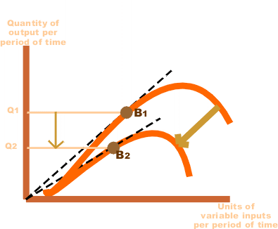
Types of production function
Short run production function
The short run is defined as the period during which at least one of the input is fixed. According to the following short-run production function, labour is the only variable factor input while the rest of the inputs are regarded as fixed. In other words, the short run is a period in which the firm can adjust production by changing variable factors such as materials and labour but cannot change fixed factors such as land, capital, etc. Thus, in short-run some factors are fixed and some are variable.
Long run production function: The long run production function is defined as the period of time in which all factors of production are variable. In the long run there is no distinction between the fixed or variable factor as all factors in the long run are variable.
The production function can also be classified on the basis of factor proportion i.e. a) Fixed proportion production function and b) Variable proportion production function.
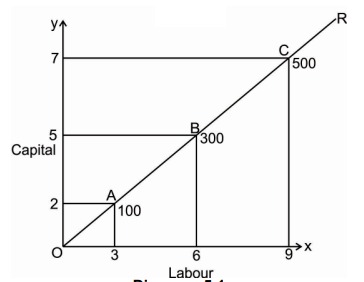
- Fixed proportion production function: The fixed proportion production function, also known as a Leontief Production Function which implies the fixed factors of production function such as land, labour, raw materials are used to produce a fixed quantity of an output and these factors of production function cannot be substituted for the other factors. In other words, in such factors of production function fixed quantity of inputs is used to produce the fixed quantity of output. All factors of production are fixed and cannot be substituted for one another. The concept of fixed proportion production function can be further expained with the help of a Diagram as shown below
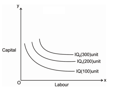
B. Variable proportion production function: The variable proportion production function supposes that the ratio in which the factors of production such as labour and capital are used in a variable proportion. Also, the different combinations of factors can be used to produce the given quantity, thus, one factor can be substituted for the other factor. In the case of variable proportion production function, the technical Coefficient of production function is variable, i.e. the important quantity of output can be achieved through the combination of different quantities of factors of production, such as these factors can be varied by substituting one factors to the other/ factors in its place. The concept of variable proportion production function can be further explained from an isoquant curve, as shown in the Diagram below:
Key takeaways - The functional relationship between the physical input (or factor of production) and therefore the output is named a production function
Law of Variable proportions
The law of variable proportion states that keeping all other factors fixed, when the quantity of one factor increased, the marginal product of that factor will eventually decline. This means that upto the use of a certain amount of variable factor, marginal product of the factor may increase and after a certain stage it starts diminishing. When the variable factor becomes relatively abundant, the marginal product may become negative.
Definition
“As the proportion of the factor in a combination of factors is increased after a point, first the marginal and then the average product of that factor will diminish.” Benham
Assumption
The following assumption of law of variable proportion
- The state of technology is assumed to be constant
- Fixed amount of other factors
- The law is based upon the possibility of varying the proportions in which the various factors can be combined to produce a product.
Illustration of the Law:
The law of variable proportion is explained in the below given table and figure. Assume that a there is a given fixed amount of land, in which more labour (variable factor) is used to produce agricultural product.
Units of labour | Total product | Marginal product | Average product |
1 | 2 | 2 | 2 |
2 | 6 | 4 | 3 |
3 | 12 | 6 | 4 |
4 | 16 | 4 | 4 |
5 | 18 | 2 | 3.6 |
6 | 18 | 0 | 3 |
7 | 14 | -4 | 2 |
8 | 8 | -6 | 1 |
In the above table we can observe that upto the use of 3 units of labour, total product increases at an increasing rate. But after the third unit total product increases at a diminishing rate.
A marginal product is the incremental change in total product as a result of increasing the variable factor i.e labour. We can see from the table, marginal product of labour initially rises and beyond the use of third unit it starts diminishing. The use of 6 units does not add anything in the production. Thus marginal product of labour fallen to zero. After the 6 unit, total product decreases and marginal product becomes negative.
Average product is derived by dividing total product by the quantity of variable unit. Till the 3 unit of labour, average product increases. Whereas after the 3 unit, average product is falling throughout.
Three Stages of the Law of Variable Proportions:
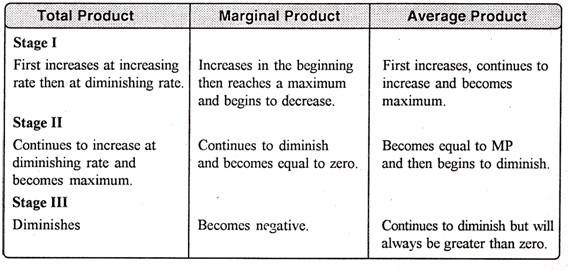
The stages are discussed in the below figure where labour is measured on the X-axis and output on the Y-axis.
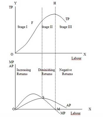
Stage 1. Stage of Increasing Returns:
In this stage, total product increases at an increasing rate till point F..ie the curve TP concave upwards upto point F which means marginal product of labour rises. Because efficiency of fixed factor increases with the increase in variable facto labour. After point F, the total product starts increasing at a diminishing rate. Looking at the next figure, marginal product of labour is maximum, after which it diminishes. This stage is called the stage of increasing returns because the average product of the variable factor labour increases throughout this stage. This stage ends at the point where the average product curve reaches its highest point.
Stage 2. Stage of Diminishing Returns:
The stage 2 ends, when the total product increases at a diminishing rate until it reaches it maximum point H. In this stage both marginal product and average product are diminishing but remain positive. Because fixed factor land becomes inadequate with the increase in the quantity of variable factor labour. At point M marginal product is zero which corresponds to the maximum point H of the total product curve.
Stage 3. Stage of Negative Returns:
In stage 3, with the increase in variable factor labour, the total product decline. Therefore the TP curve slopes downward. As a result, marginal product of labour is negative and MP cure falls below x axis. In this case fixed factor land becomes too much inadequate to the increase in variable factor labour.
Key takeaways –
- The law of variable proportion states that keeping all other factors fixed, when the quantity of one factor increased, the marginal product of that factor will eventually decline.
- Three stages are increasing return, diminishing return and negative return
Isoquants
The term “iso-quants” is derived from Greek word iso means “equal” and quants means “quantity”. Thus, iso-quant means equal quantity. An iso-quant is also known as iso-production curve, iso-indifference, equal production curve by various economists. The isoquants have its properties which are similar to those generally assumed for indifference curve theory of the theory of consumer’s behaviour analysis. Iso-quant is defined as “a locus of all the combination of two factors of production that yields that yield the same level of output.”
Thus, an iso-quant is a combination of any two factor inputs that represents and produce the same level of output. Any two combinations of input factors e.g. Labour and capital are used in which one factor is increased by decreasing the other factor of input to maintain the same level of production.
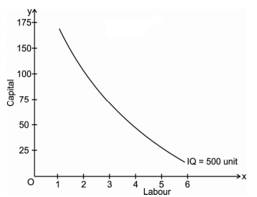
Iso-quant can be explained with the schedule and graph given below:
Factor combinations to produce a given level of output
Factor combination | Labour | Capital | Output |
A | 1 | 150 | 500 |
B | 2 | 100 | 500 |
C | 3 | 75 | 500 |
D | 4 | 50 | 500 |
E | 5 | 25 | 500 |
The above table shows the five combination of inputs i.e. Labour and Factor unit which yield the same level of output of 500 units. Which says any point on the iso-quant will give the same level of output. To show this we draw the iso-quant drawn below:
Iso-quant map:
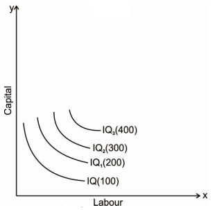
An iso-quant map represents a set of iso-quant curves shows the combination of input factor at the various level of output. A higher level of iso-quant represents the higher level of output. Thus, in simple word, iso-quant map is a family of iso-quant representing the various iso-quant curve at a particular level of output. The iso-quant map can be represented with the diagram given below:
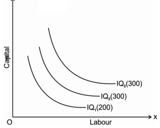
The fig above shows the various iso-quants representing the various level of output at different combination of input factors. IQ1 , IQ2 and IQ3 shows the iso-quant which produces 100,200 and 300 units of output respectively with the various combination of input factors which provides the same level of output at different level of Iso-quant.as we had said higher the Iso-quant represents higher the value of output.
Properties
- Iso-quant curve slopes downwards: The iso-quant curve slopes downwards from left to right i.e. it has a negative slope. The slope is downward because it operates under law of MRTS, when we increase labour as a factor, we have to decrease capital factor to produce a same level of output. The downward sloping iso-quant curve can be explaining the help of following Diagram
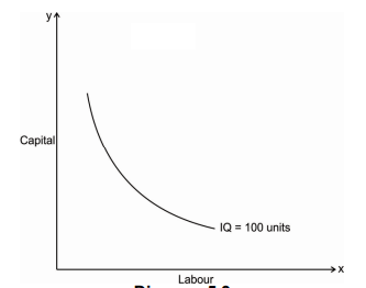
Thus, the iso-quant can be downward sloping from left to right. There can’t be an upward sloping iso-quant curve because it shows that a given product can be produce by using less of both the input factor. Similarly, an iso-quant cannot be horizontal or vertical because it also doesn’t represent the equilibrium position of a firm. Only the downward sloping supply curve represents the characteristics of iso-quant.
2. Iso-quant are convex to the origin: As we had discussed in the above property that the iso-quant curve is downward sloping and it has a negative slope and it operates under law of Marginal rate of Technical Substitution (MRTS). It says that it equals the ratio of the marginal product if labour and marginal product of capital i.e. one factor is given up to get one additional unit of other factor to produce the same of output which creates a convexity of iso-quant curve.
Thus, the slope of iso-quant can be represented by,

The above equation represents ratio of change in capital and labour should be equal to the ratio of the marginal rate of technical substitution of labour and capital which is equal to the ratio of marginal product of labour and capital.
The convexity of iso-quant means that as we move down the curve less and less of capital given up for an additional unit of labour so to produce the same level of output. The convexity of isoquant can be observed from the diagram Given below
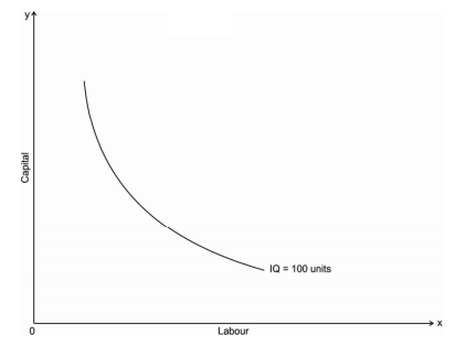
Thus, the iso-quant can be convex to the origin but not the concave because it would mean that MRTS will increase instead of decreasing i.e. labour will increase at a constant rate the amount of capital given up will goes on increasing
3. Iso-quants do not intersect: The properties of iso-quants say that two iso-quant will never intersect each other. To explain this, we will take a help of following Diagram
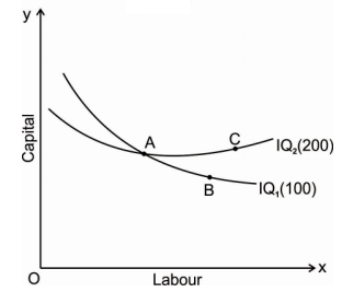
The above fig represents two different iso-quant IQ1and IQ2, where it represents the level of output 100 and 200 units respectively. Point a represents 100 units of output on IQ1 and point c represents 200 units of output on IQ2. The point b shows the intersection of both the iso-quants where is logically not possible to identify the level of output.
4. Iso-quant cannot touch either of the axis: an iso-quant cannot only touch x axis or y axis or any either axis because it will represent that the iso-quant only produce goods by using one factors of production either by using only capital or only labour which is practically not possible and which is unrealistic.
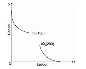
5. Higher the iso-quant higher the level of production: if there is a multiple iso-quant showing different level of production in one diagram. Where the higher the iso-quant i.e. the iso-quant far from the origin indicates higher level of output and the iso-quant close to the origin indicates lower level of output.
Return to scale
In long run, no factors are fixed. Return of scale refers to proportionate change in productivity from proportionate change in all the inputs.
Definition:
“The term returns to scale refers to the changes in output as all factors change by the same proportion.” Koutsoyiannis
“Returns to scale relates to the behaviour of total output as all inputs are varied and is a long run concept”. Leibhafsky
Types of return of scale
1. Increasing return of scale
2. Constant return of scale
3. Diminishing return of scale
Explanation
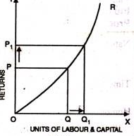
- Increasing return of scale
- When proportionate increase in factors of production leads to higher proportionate increase in production refers to increasing return of scale.
- In the below figure, x axis represent increase in labour and capital while Y axis represent increase in output. When labour and capital increases from Q to Q1, output also increases from P to P1 which is higher than the change in factors of production ie labour and capital
2. Diminishing return of scale
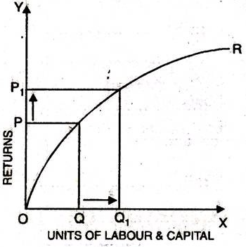
- Diminishing return refers to percentage increase in factors of proportion leads to smaller proportion increase in the output
- For instance, 30% increase in variable input (labour and capital) result in 10% increase in output.
- In the below diagram, x axis refers increase in labour and capital while Y axis refers increase in output. Percentage increase in labour and capital from Q to Q1 results in less percentage change in output from P to P1
3. Constant return of scale
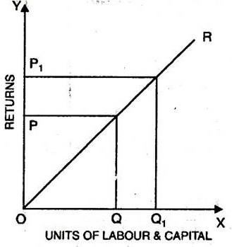
- Constant return of scale refers to output increases in same proportion in which factors of production (labour and capital) increases.
- Internal and external economies is equal to internal and external diseconomies
- This is known as homogenous production function
- In the below figure, x axis refers increase in labour and capital while Y axis refers increase in output. Increase in labour and capital from Q to Q1 is equal to the increases in output from P To P1
Key takeaways - Return of scale refers to proportionate change in productivity from proportionate change in all the inputs
Economies and Diseconomies of Scale.
Economies of scale are the factors which reduces the production cost as the volume of output increases. This means firm produces more output, then marginal cost of production decreases.
Economies of scale is divided into internal and external
Internal economies of scale – internal economies are caused by factors within the firm. It measures the company efficiency of production. The company focus on improving the output to reduce the product average cost.
Six different types of internal economies of scale: (1) technical, (2) managerial, (3) marketing, (4) financial, (5) commercial, and (6) network economies of scale.
- Technical economies of scale – this can be achieved through improvements and optimizations within the production process. When the output increases, the firm will invest more in efficient equipment and optimise operation based on experience. Efficient machinery result in producing output at lower cost.
2. Managerial economies of scale - the employment of specialised workforce result in managerial economies of scale. As the organisation grow, they hire more expert staff and create a specialised business unit. The firm efficiency is increased by employing specialist, accountants, human resource, etc which will result in reducing the cost of production and increase revenue.
3. Marketing economies of scale – marketing economies of scale is the ability to spread advertising and marketing budget over an increasing output. As the production increases the firm can fix marketing expenses, which will reduce the per unit cost of production. Better advertisement result in reaching larger audience and increase the sale of the firm.
4. Financial economies of scale – access of financial and capital market result in financial economies of scale. Large firms find easier and cheaper to raise funds. As the firm grow, it is considered to be more credit worthy. They can easily raise fund from banks, stock markets.
5. Commercial economies of scale – reduction in price due to discounts or bargaining power result in commercial economies of scale. Larger firms can buy goods and services in larger quantities. Thus they get larger discount and can bargin to negotiate lower prices. This means they pay less for each item purchases.
6. Network economies of scale - when the marginal costs of adding additional customers are extremely low result in network economies of scale. This means larger firm can support large numbers of new customers with their existing infrastructure can substantially increase profitability as they grow.
External economies of scale – external economies of scale are caused by changes outside the firm but within the industry. The factors affect the whole industry. Four different types of external economies of scale: (1) infrastructure, (2) supplier, (3) innovation, and (4) lobbying economies of scale.
- Infrastructure - public infrastructure that is put in place to benefit a specific industry result in infrastructure economies of scale. When many firms of same industry are located nearby, the government will expand infrastructure such as roads, transport, etc to meet their needs.
2. Specialization economies of scale – when suppliers and workers focus on a particular industry due to its size result in specialization economies of scale. When company within the industry increases its size and numbers, suppliers focus in that particular industry. Similarly, similarly workers find job in those industry which is growing in size.
3. Innovation economies of scale – increases public and private research result in innovation economies of scale. Industries have significant impact on the society result in growing public interest. This allows them to collaborate with research facilities and university to improve their products and processes
4. Lobbying economies of scale - Lobbying economies of scale arise from an increase in bargaining power as industries become more significant. The government is ready to compromise as these industry provide a lot of jobs and pay a significant amount of taxes.
Uneconomics of scale occurs when the long-term average cost of an organization increases. It can occur when the tissue becomes excessively large. In other words, uneconomics of Scale Causes larger org-anizations to produce goods and services at increased costs.
There are two types of scale diseconomies: internal diseconomies and external diseconomies, which are discussed as follows:
i.Internal uneconomics of the scale:
See uneconomical raising the cost of production in the organization. The main factors affecting the cost of production of the organization include the lack of determination, supervision and technical difficulties.
Ii.External uneconomics of the scale:
See uneconomical to limit the expansion of an organization or industry. Factors acting as restraints on expansion include increased production costs, a shortage of raw materials and a decline in the supply of skilled workers.
There are several causes of diseconomics of scale.
Some of the causes that lead to uneconomics of scale are:
i.Act as the main reason for diseconomics of scale.
If the organization's production goals and objectives are not properly communicated to employees in the organization, they can lead to overproduction or production. This can lead to diseconomics of scale.
Separately, if the communication process in the organization is not strong, then the employee will not get enough feedback. As a result, there will be less face-to-face interaction between employees, which will affect the production process.
Ii.Lack of motivation:
This leads to a decrease in productivity levels. For large organizations, workers may feel isolated and less motivated because they are less valued for their work. Because of poor communication networks, it is difficult for employers to interact with employees and build a sense of attributes. This leads to a decrease in the productivity level of output due to lack of motivation. This further leads to an increase in the cost of the organization.
Iii.Loss of control:
It serves as the main problem of large organizations. Monitoring and controlling the work of all employees in a large organization becomes impossible and expensive. It is difficult to make sure that all employees of the organization are working towards the same goal. It becomes difficult for managers to direct the sub-coordinates of large organizations.
Iv.Cannibalism:
It means a situation where an organization is facing competition from its products. While smaller organizations face competition from the products of other organizations, larger organizations find their products compete with each other.
Case Study and Analysis of the Production Processes in a Steel Factoryin Jordan
This work represents a true case study and analysis of the technical and energy managerial aspects of recommended designs of the production lines of a steel factory in Jordan. A modern structure of a control system based on SCADA (Supervisory Control And Data Acquisition) technology is proposed. Furthermore, the mechanical and electrical maintenance sections in the factory were reviewed due to their major effects on the production cost and energy consumption of the factory. This study was performed in two main phases: The first phase contains the collected data and process assessment that were undertaken by traditional direct observation and activity categorization, while the second phase gave details on the proposed control methodology in terms of design and architecture.
Moreover, a proposal on maintenance planning and procedure program was also included in this study in order to reduce the time and accordingly the cost of maintenance. The steel factory studied produces various steel products such as: Concrete Reinforcement Steel Bars (Rebars), Flat & Square Bars Section which includes standard flat bars, standard square bars, and plane round bars, in addition to Wire mesh in different sizes and steel billets. In steel production industries, two automation levels can, in general, be identified. The first level involves the electromechanical actuation of the devices in the production plant; this level of automation is currently available in every plant. The second level involves the supervision of the production process; this level of automation is less frequent and is generally only partial. In fact, steel production involves a variety of complex physical phenomena, described by sophisticated mathematical models which are rarely usable to derive real -time advice for process supervision and control. Most operators' support systems for steel production are represented by simple technologies such as microprocessor-based systems.
Based on the outcomes of this study, the factory purchased a new melting furnace of (60) tons capacity instead of the (30) tons capacity melting furnace used in the factory before the study. The factory is considering also the purchase of a scrap press in its new budget in order to improve scrap quality before melting it; in order to reduce the rate of consuming the furnace electrodes. Also, the maintenance section will be restructured by merging electrical and mechanical maintenance sections into one section headed by the deputy of the factory manager.
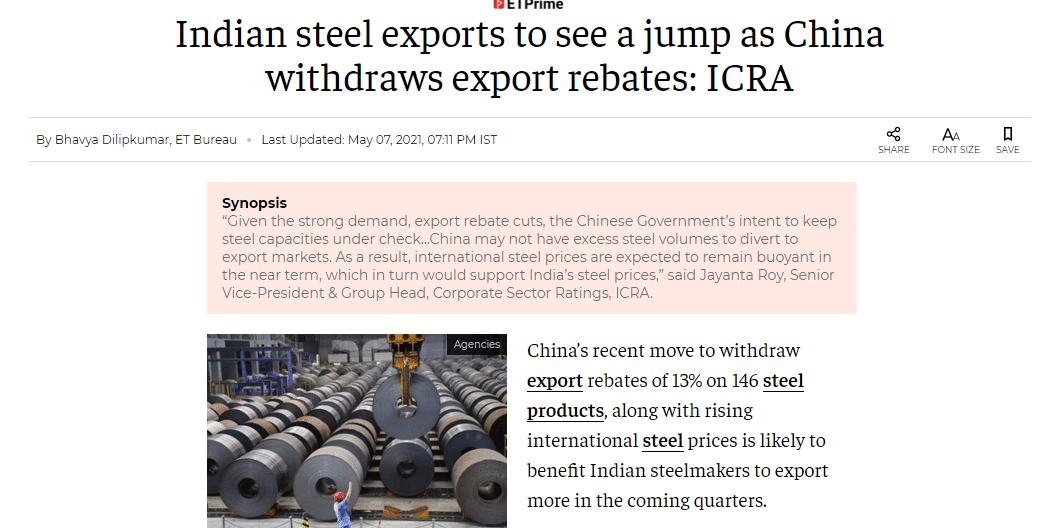
News
Concept of cost
A firm who wants to maximize their profit concentrates on revenue and cost of the firm. Profit of the firm can be increased either by increasing revenue or by reducing cost. Firm generally cannot influence revenue because it is determined by the market forces but it is possible for the firm to reduce cost by producing maximum output or by increasing efficiency of the organization.
For managerial decision-making, cost is very important because it helps to decide price for the commodity. It also helps to decide whether to increase the production or not. Therefore, understanding of cost concepts is very important.
- Private cost and Social cost: Costs which are directly incurred by the individual or firm producing good or service is called private cost. This cost gives private benefit to an individual or firm engaged in relevant activity. Some of the examples of private cost are firm’s expenditure on purchase of raw material, payment of rent, wages and salaries, interest, insurance, depreciation etc. Similarly company’s expenditure for its labor, advertising cost for the promotion of goods, transportation cost to carry goods from company to the market are also considered as private cost.
Social cost on the other hand is bared by the society as a result of production of commodity. Even though social cost occurs due to production of a commodity it is not bared by the producer. It consists of external cost. E.g.: If a factory is located in a residential area causes air pollution. Due to pollution as the health of the people living in that area affects, they have to spend money on medical facilities. Even though this cost occurs due to the factory, it is passed on to the society at large. Externalities are included in the social cost
b. Historical cost and Replacement cost: The original money value spent at the time of purchasing of an asset is called historical cost. Most of the assets in the balance sheet are at the historical cost. One of the advantages of historical cost is that records maintained on the basis of historical cost are considered to be reliable, consistent, comparable and verifiable. Historical cost does not reflect current market valuation.
The amount which has to be spent at the time of replacing of the existing asset is called the replacement cost. This cost reflects the current market prices. If we consider an increase in prices over the years, replacement cost will be greater than historical cost. If we consider fall in prices over the years, replacement cost will be less than historical cost and if we consider prices to be constant over the years, replacement cost and historical costs are the same.
c. Fixed cost and Variable cost: Fixed cost refers to the firm’s expenditure on fixed factors of production. Even if no output is produced, fixed cost needs to be paid. Even if output increases in the short run, fixed cost remains constant. E.g.: If a businessman borrows money from a bank to start his business. Initially even if his output is zero, he has to pay the interest on borrowed capital. Rent on land, insurance premium, tax payment are some of the examples of fixed cost. Addition of all fixed cost gives Total Fixed Cost.
Variable cost on the other hand refers to the firm’s expenditure on variable factors of production. When no output is produced, variable cost is zero. As output increases, variable cost also increases. Payment for raw material, wages and salaries of the workers are some of the examples of variable cost. Addition of all variable costs gives the Total Variable Cost.
d. Total cost, Average cost and Marginal cost: Total cost (TC) – Firms total expenditure on all fixed and variable factors for producing a commodity is called the Total cost of production. Therefore TC= TFC+TVC For zero level of output there is some total cost. It increases with an increase in the level of output
Average Cost (AC) or Average Total Cost (ATC) – It refers to the per unit cost of producing a commodity. It is calculated by the following formula
AC = TC/Q
Where AC = Average cost TC = Total cost Q = Number of units produced
Average cost can also be calculated by using following formula
AC or ATC = AFC+AVC
Where AC- Average Cost AFC- Average Fixed Cost AVC- Average Variable Cost
Average Fixed Cost (AFC)- It is the per unit fixed cost of production. It can be calculated by the following formula
AFC= TFC/Q
Where TFC= Total Fixed Cost Q = Number of units produced
Average Variable Cost (AVC) - It is the per unit variable cost of production. It can be calculated by the following formula
AVC= TVC/Q
Where TVC= Total Variable Cost Q= Number of units produced
Marginal Cost (MC) - It is the addition made to the total cost. Or cost of producing an additional unit of output is called as the marginal cost. It can be calculated by using following formula
MC = Change in total cost/ change in output TC
Eg: If total cost of producing 2 cars is Rs. 3, 00,000 and the total cost of producing 3 cars is Rs. 4, 50,000. Then the marginal cost is Rs. 1, 50,000 i.e. the cost of producing an additional unit of output.
e. Sunk Cost and Incremental Cost: In order to enter in to the market certain costs are incurred by the firm. These costs are known as Sunk cost. It includes the cost by the firm for setting up the business, advertisement etc. These costs cannot be recovered by the firm if they decide to exit the market.
Incremental cost refers to a change in total coat as a result of policy change or a change in managerial decision. The concept of incremental cost is broader as compared to marginal cost.
Marginal cost considers a change in total cost due to a unit change in output whereas incremental cost considers a change in total cost due to an introduction of new product, change in advertising strategy, additional batch of output etc. The concept of incremental cost is more relevant as compared to marginal cost because the firm increases its output in batches and not by unit only.
f. Implicit Cost and Explicit Cost: Implicit cost refers to the cost of all own factors which the entrepreneur employs in the business. It includes salary and wages for the service of entrepreneur, interest on capital invested by the entrepreneur etc. Implicit costs are also called indirect cost because direct cash payment is not made to own factors of production.
If entrepreneur sold these services to others, he would have earned money. Therefore, implicit cost is also the opportunity cost of factors owned by him.
Explicit cost on the other hand is the direct cash payment made by the firm for purchasing or hiring of various factors of production. E.g. Rent paid for hiring of land, money spent for purchasing for raw material, wages and salaries paid to the employees, expenditure on transport, power, advertising etc.
g. Accounting and Economic Cost: Accounting cost includes only explicit cost i.e. the firm’s expenditure on purchasing of various factors of production. For financial purpose and tax purpose, accounting cost is important.
Economic cost on the other hand includes both explicit and implicit cost. This cost is important for managerial decision making. Therefore an economist who wants to take any decision considers both explicit and implicit cost.
Long run and short run cost of production
Cost behavior in the short term
Short-term costs are important for understanding costs in economics. Short-term and long-term distinctions based on fixed and variable factors of production make the concept of understanding short-term costs easier. Let us understand the concept using examples, diagrams for graphical representation.
Short run concept
To understand short-term costs, it is important to understand the concept of short-term costs. In economics, we distinguish between short-term and long-term through the application of fixed or variable inputs.
Fixed input (plant, machine, etc.)) is a factor of production that can not be changed or changed in a short span because the period is"too small". This will be short-term. Here, the inputs are two types: fixed and variable.
In the long run, all inputs will be mutable(e.g.. Raw materials). This means that all inputs can be changed as the output volume changes. Therefore, the concept of fixed input applies only in the short term. It is in the short-term cost that we turn this time.
It explains that the cost of production depends on the level of output, given that others remain the same (ceteris paribus). This can be mathematically written as:
C=f(X)
Where C is the production cost and X is the output level.
Total fixed costs
Fixed cost refers to the cost of fixed input. At the level of output it does not change (hence, fixed). Fixed inputs include buildings,machines, etc. Thus, the cost of inputs, such as rent and the cost of machines, constitute a fixed cost. Also known as overhead, supplemental or overhead, these costs remain the same regardless of the level of output.
So if you plot the total fixed cost (TFC) curve against the output level on the horizontal axis, you get a straight line parallel to the horizontal axis. This indicates that these costs remain the same and should occur even if the output level is zero.
Total variable costs
The costs incurred by variable factors in production are called Total variable costs(TVC). These costs differ in the level of output. Therefore, when the production level is zero, the TVC is also zero. Thus, the TVC curve begins at the origin.
The Shape of the TVC is unique. It is said that it has the form of an inverted S. This is because, in the early stages of production, there is a scope for efficient use of fixed factors by using more variable factors (e.g., variable factors). Workers who use the machine).
Thus, as the variable input used increases, the production efficiency of the variable input ensures at a rate at which the TVC increases but decreases. This makes the first part of the tvc curve concave.
As production continues to increase, more variable factors are employed for a given amount of fixed inputs. The production efficiency of each variable factor is reduced,adding more to the production cost. Therefore, TVC will increase,but now it is increasing at the rate of increase. This is where the shape of the TVC curve is convex. Thus, the TVC curve will have an inverted-S shape.
Total cost
Total cost(TC) refers to the sum of fixed and variable costs incurred in the short term. So, the short-term cost can be expressed as follows
TC=TFC+TVC
Note that in the long run, TFC=0, so TC = TVC. So you can get the shape of the TC curve by summing the TFC curve and the TVC curve.
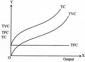
For the TC curve, the following points can be noted:
- The TC curve is shaped of reverse S. This is because of the TVC curve. Since the TFC curve is horizontal, the difference between the TC curve and the TVC curve is the same at each level of the output and is equal to the tfc. This is explained as follows: TC-TVC=TFC
- The TFC curve is parallel to the horizontal axis, and the TVC curve is inverted S-shaped.
- The law that explains the Shape of TVC and subsequent TC is called the law of variable proportions.
Profit maximisation and cost minimization
Cost Minimisation for a Given Output:
In the theory of production, the profit maximisation firm is in equilibrium when, given the cost- price function, it maximises its profits on the basis of the least cost combination of factors. For this, it will choose that combination which minimises its cost of production for a given output. This will be the optimal combination for it.
Assumptions:
1. There are two factors, labour and capital.
2. All units of labour and capital are homogeneous.
3. The prices of units of labour (w) and that of capital (r) are given and constant.
4. The cost outlay is given.
5. The firm produces a single product.
6. The price of the product is given and constant.
7. The firm aims at profit maximisation.
8. There is perfect competition in the factor market.
Explanation:
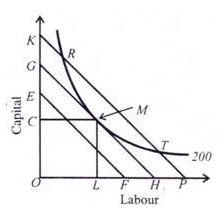
Given these assumptions, the point of least-cost combination of factors for a given level of output is where the isoquant curve is tangent to an isocost line. In Figure ,the isocost line GH is tangent to the isoquant 200 at point M. The firm employs the combination of ОС of capital and OL of labour to produce 200 units of output at point M with the given cost-outlay GH.
At this point, the firm is minimising its cost for producing 200 units. Any other combination on the isoquant 200, such as R or T, is on the higher isocost line KP which shows higher cost of production. The isocost line EF shows lower cost but output 200 cannot be attained with it. Therefore, the firm will choose the minimum cost point M which is the least-cost factor combination for producing 200 units of output. M is thus the optimal combination for the firm.
The point of tangency between the isocost line and the isoquant is an important first order condition but not a necessary condition for the producer’s equilibrium.
There are two essential К or second order conditions for the equilibrium of the firm:
- The first condition is that the slope of the isocost line must equal the slope of the isoquant curve. The slope of the isocost line is equal to the ratio of the price of labour (w) and the price of capital (r). The slope of the isoquant curve is equal to the marginal rate of technical substitution of labour and capital (MRTSlk ) which is, in turn, equal to the ratio of the marginal product of labour to the marginal product of capital (MPl/MPk‘ condition for optimality can be written as.

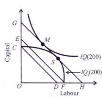
The second condition is that at the point of tangency, the isoquant curve must be convex to the origin. In other words, the marginal rate of technical substitution of labour for capital (MRTSlk) must be diminishing at the point of tangency for equilibrium to be stable. In second Figure below, S cannot be the point of equilibrium for the isoquant IQ is concave where it is tangent to the isocost line GH. At point S, the marginal rate of technical substitution between the two factors increases if move to the right or left on the curve IQl.
Moreover, the same output level can be produced at a lower cost AB or EF and there will be a comer solution either at С or F. If it decides to produce at EF cost, it can produce the entire output with only OF labour. If, on the other hand, it decides to produce at a still lower cost CD, the entire output can be produced with only ОС capital.
Both the situations are impossibilities because nothing can be produced either with only labour or only capital. Therefore, the firm can produce the same level of output at point M, where the isoquant curve IQ is convex to the origin and is tangent to the isocost line GH. The analysis assumes that both the isoquants represent equal level of output, IQ = IQ1.
Output-Maximisation for a Given Cost:
The firm also maximises its profits by maximising its output, given its cost outlay and the prices of the two factors. This analysis is based on the same assumptions, as given above. The conditions for the equilibrium of the firm are the same, as discussed above.
- The firm is in equilibrium at point Р where the isoquant curve 200 is tangent to the isocost line CL in Figure below. At this point, the firm is maximising its output level of 200 units by employing the optimal combination of OM of capital and ON of labour, given its cost outlay CL.
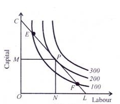
But it cannot be at points E or F on the isocost line CL, since both points give a smaller quantity of output, being on the isoquant 100, than on the isoquant 200. The firm can reach the optimal factor combination level of maximum output by moving along the isocost line CL from either point E or F to point P.
This movement involves no extra cost because the firm remains on the same isocost line. The firm cannot attain a higher level of output such as isoquant 300 because of the cost constraint. Thus the equilibrium point has to be P with optimal factor combination OM+ ON. At point P, the slope of the isoquant curve 200 is equal to the slope of the isocost line CL. It implies w/r = МРL/МРK = MRTSLK.
2. The second condition is that the isoquant curve must be convex to the origin at the point of tangency with the isocost line
Equilibrium of the firm
“A firm is a unit engaged in the production for sale at a profit and with the objective of maximizing profit.” –Watson
Onditions of the Equilibrium of Firm:
A firm is said to be in equilibrium when it satisfies the following conditions:
1. The first condition for the equilibrium of the firm is that its profit should be maximum.
2. Marginal cost should be equal to marginal revenue.
3. MC must cut MR from below.
The above conditions of the equilibrium of the firm can be examined in two ways:
1. Total Revenue and Total Cost Approach:
A firm is said to be in equilibrium when it maximizes its profit. It is the point when it has no tendency either to increase or contract its output. Now, profits are the difference between total revenue and total cost. So in order to be in equilibrium, the firm will attempt to maximize the difference between total revenue and total costs. It is clear from the figure that the largest profits which the firm could make will be earned when the vertical distance between the total cost and total revenue is greatest.
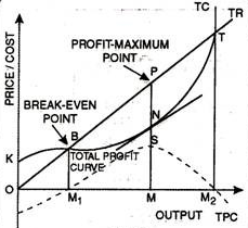
In fig. Above output has been measured on X-axis while price/cost on Y-axis. TR is the total revenue curve. It is a straight line bisecting the origin at 45°. It signifies that price of the commodity is fixed. Such a situation exists only under perfect competition.
TC is the total cost curve. TPC is the total profit curve. Up to OM1 level of output, TC curve lies above TR curve. It is the loss zone. At OM1 output, the firm just covers costs TR=TC. Point B indicates zero profit. It is called the break-even point. Beyond OM1 output, the difference between TR and TC is positive up to OM2 level of output. The firm makes maximum profits at OM output because the vertical distance between TR and TC curves (PN) is maximum.
The tangent at point N on TC curve is parallel to the TR curve. The behaviour of total profits is shown by the dotted curve. Total profits are maximum at OM output. At OM2 output TC is again equal to TR. Profits fall to zero. Losses are minimum at OM] output. The firm has crossed the loss zone and is about to enter the profit zone. It is signified by the break-even point-B.
2. Marginal Revenue and Marginal Cost Approach:
Joan Robinson used the tools of marginal revenue and marginal cost to demonstrate the equilibrium of the firm. According to this method, the profits of a firm can be estimated by calculating the marginal revenue and marginal cost at different levels of output. Marginal revenue is the difference made to total revenue by selling one unit of output. Similarly, marginal cost is the difference made to total cost by producing one unit of output. The profits of a firm will be maximum at that level of output whose marginal cost is equal to marginal revenue.
Thus, every firm will increase output till marginal revenue is greater than marginal cost. On the other hand, if marginal cost happens to be greater than marginal revenue the firm will sustain losses. Thus, it will be in the interest of the firm to contract the output. It can be shown with the help of a figure. In below fig MC is the upward sloping marginal cost curve and MR is the downward sloping marginal revenue curve. Both these curves intersect each other at point E which determines the OX level of output. At OX level of output marginal revenue is just equal to marginal cost.
It means, firm will be maximizing its profits by producing OX output. Now, if the firm produces output less or more than OX, its profits will be less. For instance, at OX1 its profits will be less because here MR = JX1, while MC = KX1 So, MR > MC. In the same fashion at OX2 level of output marginal revenue is less than marginal cost. Therefore, beyond OX level of output extra units will add more to cost than to revenue and, thus, the firm will be incurring a loss on these extra units.
Besides first condition, the second order condition must also be satisfied, if we want to be in a stable equilibrium position. The second order condition requires that for a firm to be in equilibrium marginal cost curve must cut marginal revenue curve from below. If, at the point of equality, MC curve cuts the MR curve from above, then beyond the point of equality MC would be lower than MR and, therefore, it will be in the interest of the producer to expand output beyond this equality point. This can be made clear with the help of the figure.
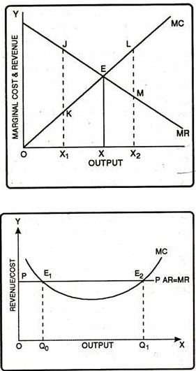
In second figure output has been measured on X-axis while revenue on Y-axis. MC is the marginal cost curve. PP curve represents the average revenue as well as marginal revenue curve. It is clear from the figure that initially MC curve cuts the MR curve at point E1. Point E1 is called the ‘Break Even Point’ as MC curve intersects the MR curve from above. The profit maximizing output is OQ1 because with this output marginal cost is equal to marginal revenue (E2) and MC curve intersects the MR curve from below.
Technology Change in the very long run
The long run is the period of time when all costs are variable. The long run depends on the specifics of the firm in question—it is not a precise period of time. If you have a one-year lease on your factory, then the long run is any period longer than a year, since after a year you are no longer bound by the lease. No costs are fixed in the long run. A firm can build new factories and purchase new machinery, or it can close existing facilities. In planning for the long run, the firm will compare alternative production technologies (or processes).
In this context, technology refers to all alternative methods of combining inputs to produce outputs. It does not refer to a specific new invention like the tablet computer. The firm will search for the production technology that allows it to produce the desired level of output at the lowest cost. After all, lower costs lead to higher profits—at least if total revenues remain unchanged. Moreover, each firm must fear that if it does not seek out the lowest-cost methods of production, then it may lose sales to competitor firms that find a way to produce and sell for less.
Sources
- Pindyck, R.S. , D.L. Rubinfield and P.L. Mehta; Microeconomics, Pearson Education.
- N. Gregory mankiw, Principles of Micro Economics, Cengage Learning
- Browining E.K. And J.M. Browining: Microeconomics Theory and Applications, Kalyani Publishers, New Delhi.
- Gould, J.P and E.P. Lazear: Microeconomics Theory, All India Traveller Bookseller New Delhi