UNIT 5
Income Distribution and Factor Pricing
Demand for a Factor:
Let us first consider the demand side. In the first place, we should remember that the demand for a factor of production is not a direct demand if is an indirect or derived demand. It is derived from the demand for the produce that the factor produces. For instance, labour does not satisfy our wants directly. We want labour for the sake of the goods that it produces. It follows, therefore, that if the demand for goods increases, the demand for the factors which help to produce these goods will also increase. Also, if the demand for goods is elastic or inelastic, the demand for the factors too will be elastic or inelastic.
The demand for a factor of production will also depend on the quantity of the other factors required in the process. Generally speaking, the demand price for a given quantity of a factor of production will be higher, the greater the quantities of the co-operating productive services. If more of a factor of production is employed, the marginal productivity of the factor will fall, and the lower will be the demand price for the unit of a productive service. This is another rule connected with the demand for a factor of production.
The demand price of a factor of production also depends on the value of the finished product in the production of which the factor is used. The demand price will generally be greater; the more valuable is the finished product in which the factor is used. Also, the more productive the factor, he higher will be the demand price of a given quantity of the factor.
These are a few points connected with the demand for a productive service. We know that the demand curve of the industry is the sum-total of the demand curves of the various firms in the industry. By a similar summing up, we can have the demand curve of all the industries using a particular productive service.
The demand of the employer for a factor depends on its marginal revenue productivity (in short, marginal productivity), and the quantity of the factor that a firm will employ will depend on the prevailing wage-level. That is more labour will be employed if wages are low and less if wages are high.
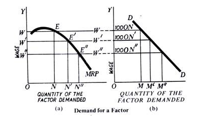
In the below fgure (a) illustrates the position of a firm regarding the employment of a factor, say, labour. When the wage is OW, the firm is in equilibrium at the point E and the demand for the factor is ON; similarly, at OW’ wage, the demand is ON’, and at OW” the demand is ON”. MRP (marginal revenue productivity) curve is the demand curve for a factor of production by an individual firm.

But for determining the price of a factor, it is not the demand of the individual firm for it that matters. What matters is the total demand, i.e., the sum-total of the demands of all firms in the industry. The total demand curve is derived by the lateral summation of the marginal revenue productivity curves of all the firms. This curve DD is shown in the above Fig.(b).
It can be seen that Y-axes in both curves are drawn to the same scale, but X-axes are drawn on different scales. We have supposed that there are 100 firms in the industry. At OW wage, the demand of the individual firm is ON, but the demand of the whole industry at the same wages is OM, which is equal to 100 ON (because the number of firms in the industry is 100). In the same manner, at OW’ the demand of the firm is ON’ but of the entire industry OM’, which is equal to 100 ON’, and at OW”, the demand of the firm is ON” and that of the industry OM”, which is equal to 100 ON”.
It can be seen that the demand curve DD slopes downward to the right. The reason is that MRP curve, whose summation is represented by DD, also slopes down similarly to the right in the relevant portion. This means that according to the law of diminishing marginal productivity, the more a factor is employed the lower is the marginal productivity. This is all about the demand side.
Supply Side:
As for the supply side, the supply curve of a factor depends on the various conditions of its supply. Take the case of labour—a very important productive service. The supply of labour will depend on the size and composition of population, its occupational and geographical distribution, labour efficiency, cost of education and training, cost of movement, the expected income, relative preference for work and leisure, and so on. In this manner, by considering all the relevant factors, it is possible to construct the supply curve of a productive service.
At the same time, we must note that the supply is a bit of complicated thing. We generally say that the supply of land is limited. But the fact is that, although for the whole community land is limited, for a particular firm or an industry, its supply is not limited. The supply can be increased if higher rent is offered.
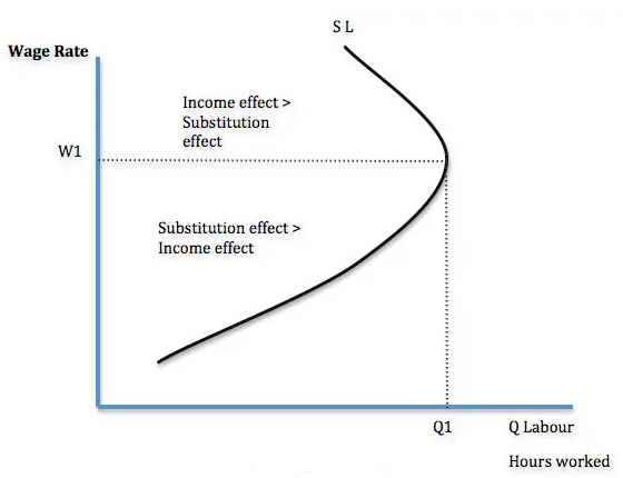
In the case of commodities, we see that generally an increase in price brings forth larger supplies. This, however, does not necessarily hold good in the case of the factors of production. It may happen in some cases that, if wags go up, labour may be able to satisfy its needs by working for less time than before. They may prefer leisure to work. In this case, when the price of factor (or its remuneration) is increased, the supply is reduced. This peculiarity will be represented by a backward sloping curve after a stage.
Also, the supply of labour does not merely depend on economic factors; many non-economic considerations also enter. All the same, we can say that, if the price of a factor increases, its supply will also generally increase, and vice versa. Hence, the supply curve of a factor rises from left to right upwards. This is shown in the below fig.

Interaction of Demand and Supply:
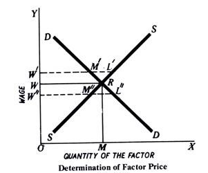
Now we have worked our way to the demand curve and the supply curve of a factor of production. Both these curves are needed for the determination of the price of a productive service. That price will tend to prevail in the factor market at which the demand and supply are in equilibrium. This equilibrium is at the point of intersection of the demand and supply curves.
In the second they intersect at the point R, and the price of the factor will be OW. At OW’ demand W’M’ is less than the supply W’L’. In this case, competition among the sellers of the service will tend to bring down the price to OW. On the other hand, at OW” price, the demand W”L” is greater than the supply W”M”; hence price will tend to go up to OW at which the demand and supply will be equal.
This is how the price of a factor of production in the factor market is determined by the interaction of the forces of demand and supply relating to that factor of production.
Key takeaways –
- The marginal product of a labour in any industry is the amount by which the output would be increased if a unit of labour was increased, while the quantities of other factors of production remaining constant.
In economics, a backward-bending supply curve of labour, or backward-bending labour supply curve, is a graphical device showing a situation in which as real (inflation-corrected) wages increase beyond a certain level, people will substitute leisure (non-paid time) for paid work time and so higher wages lead to a decrease in the labour supply and so less labour-time being offered for sale. The "labour-leisure" tradeoff is the tradeoff faced by wage-earning human beings between the amounts of time spent engaged in wage-paying work (assumed to be unpleasant) and satisfaction generating unpaid time, which allows participation in "leisure" activities and the use of time to do necessary self-maintenance, such as sleep. The key to the tradeoff is a comparison between the wage received from each hour of working and the amount of satisfaction generated by the use of unpaid time. Such a comparison generally means that a higher wage entices people to spend more time working for pay; the substitution effect implies a positively sloped labour supply curve. However, the backward-bending labour supply curve occurs when an even higher wage actually entices people to work less and consume more leisure or unpaid time.
A typical supply curve shows an increase in supply as wages rise. It slopes from left to right.
However, in labour markets, we can often witness a backward bending supply curve. This means after a certain point, higher wages can lead to a decline in labour supply. This occurs when higher wages encourage workers to work less and enjoy more leisure time.

There are two effects related to determining supply of labour.
- The substitution effect states that a higher wage makes work more attractive than leisure. Therefore, in response to higher wages, supply increases because work gives greater remuneration.
- The income effect states that a higher wage means workers can achieve a target income by working fewer hours. Therefore, if wages increase, it becomes easier to get enough income through working fewer hours.
Key takeaways –
- The backward-bending labour supply curve occurs when an even higher wage actually entices people to work less and consume more leisure or unpaid time.
Functional distribution refers to the distinct share of the national income received by the people, as agents of production per Unit of time, as a reward for the unique functions rendered by them through their productive services. These shares are commonly described as wages, rent, interest and profits in the aggregate production. It implies factor price determination of a class of factors. It has been called as “Macro” concept.
The functional distribution of income refers to the amounts of income paid to various individuals or households. A single individual may receive income from more than one factor of production or from one source. A man may get income by offering his labour service, from renting his property (land or building) and from his holdings of company shares or government bonds.
When income is classified according to the size of income received by each households irrespective of the sources of that income, we are dealing with the size distribution of income. Progressive income taxes are imposed and subsidies are paid to reduce income inequality.
According to neo-classical theory, the income of any factor of production (and hence the amount of the national product that it is able to command) depends on the price that is paid for the factor and the amount that is purchased or hired.
For instance, total wage income = the wage rate x the number of workers employed. Thus factor pricing and income distribution are interrelated. If the wage rate rises and more workers are employed at a higher wage, the share of labour in national income will also rise and workers will now be able to buy those things which they could not previously afford.
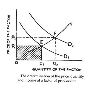
The market price of any commodity like carrots is determined by the impersonal forces of demand and supply. In Fig. Below the demand and supply curves for some factor of production are D1 and S. The equilibrium price and quantity are p1 and q1, respectively. The total income earned by the factor is indicated by the area Op1Eq1 (which is op1 x oq1).

Our analysis of factor-pricing and income distribution is based on the assumption that the prices of all other factors of production the prices of all goods, and the level of national income are given constants’ Fluctuations in the equilibrium price and quantity may cause fluctuations in the return to the factor, in its relative earnings (compared to other factors) and in the share of national income going to the factor.
Suppose, for instance that the demand curve for the factor in question shifts from D1 to D2. Now the price of the factor rises from P1 to p2 and the relative price rises from p1/f to p2/f where f is the given average price of all other factors.
The total earnings rise from p1q2 to p2q2 and if the total income in the whole economy remains constant at a then the share of income going to this factor rises from P1q1/a to p2q2/a. This is the essence of the free-market determination of a factor’s price and its share of national income.
Key takeaways –
- The functional distribution of income refers to the amounts of income paid to various individuals or households.
Sources
- Pindyck, R.S. , D.L. Rubinfield and P.L. Mehta; Microeconomics, Pearson Education.
- N. Gregory mankiw, Principles of Micro Economics, Cengage Learning
- Browining E.K. And J.M. Browining: Microeconomics Theory and Applications, Kalyani Publishers, New Delhi.
- Gould, J.P and E.P. Lazear: Microeconomics Theory, All India Traveller Bookseller New Delhi