Unit - 9

Microsoft Excel (Spreadsheet)

9.1 Spreadsheet Concepts, Creating, Saving and Editing a Workbook

In Excel, a file is referred to as a "Workbook." A workbook is made up of several “Worksheets” (Fig). Users have access to three sheets by default: Sheet 1, Sheet 2, and Sheet 3. Only one worksheet can be designated as a "Active Worksheet" at a time, and that worksheet is available to the user for actions. The name of an active worksheet appears in bold characters in the "Sheet Tab" at the bottom left of the screen. If necessary, additional sheets can be added by clicking the icon (which operates as Insert! Worksheet).

If necessary, the sheet names can be changed by right-clicking the mouse above Sheet1 or Sheet 2 or Sheet 3 after selecting and directing it on the sheet name to be changed and selecting “Rename.”

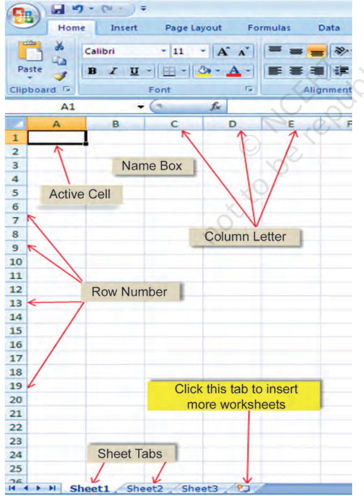
Columns are referred to by alpha characters from left to right, while rows are numbered numerically from top to bottom. There are 65536 rows in Excel 2007 that are numbered 1, 2, 3,... 65,536. These figures can be seen on the worksheet's left-hand side. Columns (a total of 256 in Excel) are labeled with letters such as A, B, C,... AA... IV and are displayed on the horizontal box right above Row 1. As a result, there are roughly 65,536 x 256 = 1,65,00,000 cells, which is a large work surface, sufficient for all application requirements (Fig) on a single sheet.

A cell in a spreadsheet stores a value, function, or arithmetic expression. A cell is the point where a row and a column meet. A cell is designated by a letter and a number combination that corresponds to a specific location inside the spreadsheet. For example, as seen in Figure at row 1 and column 1, the first cell in a worksheet is designated as A1 (A).

Creating

Workbooks are Excel documents. We'll need to generate a new workbook every time we start a new project in Excel. In Excel 2016, there are several ways to begin working with a workbook. We can either start from scratch or use a predesigned template to create a new worksheet, or we can open an existing one.

Create a new blank workbook

Follow these procedures to create a fresh blank workbook in MS Excel:

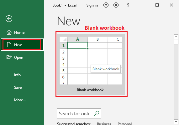
1. Go to the File tab, where you'll see the Excel Backstage view.

2. Choose New, then Blank Workbook from the drop-down menu.

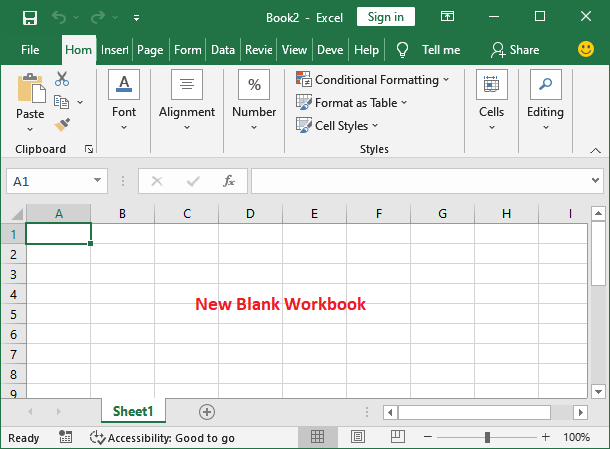
3. This will result in the creation of a new blank workbook.

Saving and Editing a workbook

We'll need to know how to save a new worksheet in Excel so that we can access and edit it later. We can save files locally on our computer, just like in previous versions of Excel. Unlike previous versions, however, Excel 2016 allows us to save a worksheet to the cloud using OneDrive.

Additionally, Excel allows us to immediately export and share workbooks with others.

Save and Save as

Save and Save As are the two options for saving a file in Excel. These choices operate in a similar manner, with a few key distinctions:

Save - We'll use the Save command to save our changes when we create or modify a worksheet. The majority of the time, we'll utilize this command.

Only when saving a file for the first time do we need to choose a file name and location. After that, we can simply save it with a same name and location by clicking the Save command. You can also use the Ctrl+S keyboard shortcut.

Save as - This command will be used to make a copy of a workbook while maintaining the original. When we use Save As, we must provide the cloned version a different name and/or location.

Steps to save a workbook

Every time we start a new project or make changes to an existing one, we must save our workbook. Early and frequent saving can help us avoid losing our work.

1. On the Quick Access Toolbar, locate and pick the Save command.

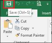
2. The Save As pane will appear in the Backstage view if we're saving the file for the first time. Choose a new file name and a new location to save your file.

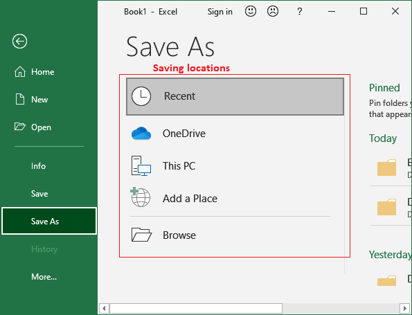
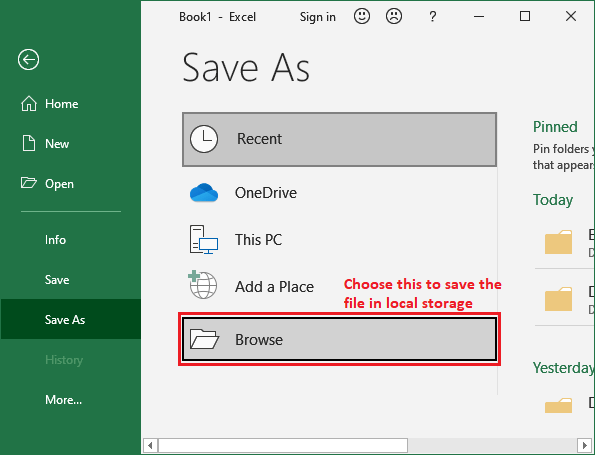
3. Click the Browse button here to save the workbook to our computer. Alternatively, we can save the file to your OneDrive by clicking OneDrive.

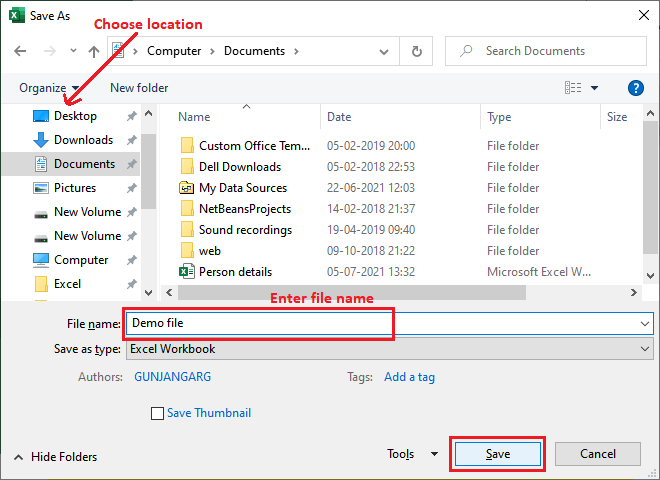
4. You'll see the Save As dialog box appear. Select the place in local storage where the workbook should be saved. Click Save after you've given the workbook a name.

5. You'll save the worksheet. As we make changes to the worksheet, we may use the Save command (Ctrl+S) to save our modifications.

9.2 Inserting

Using pre-made Excel workbooks is a time-saving method of working because it avoids the need to construct data worksheets from scratch. However, you may discover that you need to add more columns or rows of data to achieve your objectives. In this situation, you can create a worksheet with blank columns or rows. The steps below will show you how to do it:

1. By hovering the mouse pointer over cell C1 in the Sheet1 worksheet and clicking the left mouse button, you can access it.
2. In the Home tab of the Ribbon, click the down arrow on the Insert button.

3.     From the drop-down menu, select Insert Sheet Columns. To the left of Column C, a blank column will be added. Column D now contains the contents that were previously in Column C. It's worth noting that columns are always placed to the left of an activated cell.

4.     By hovering the mouse pointer over cell A3 in the Sheet1 worksheet and clicking the left mouse button, you can access it.

5.     In the Home tab of the Ribbon, click the down arrow on the Insert button.

6.     From the drop-down menu, select the Insert Sheet Rows option. Above Row 3, a blank row will be inserted. Row 4 now contains the contents that were previously in Row 3. It's important to note that rows are always placed above the activated cell.

9.3 Deleting Worksheets

1. Select Delete from the worksheet menu after right-clicking the worksheet you want to remove.

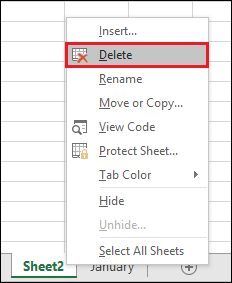
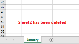
2.     The targeted worksheet has been removed from our workbook, as you can see. There is only one worksheet left.

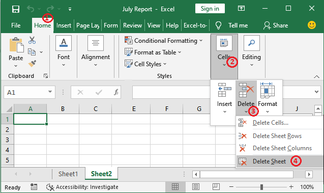
You can also go to the Cells Group's Home Tab, click Delete, and then pick Delete Sheet.

9.4 Entering data in a cell / formula Copying and Moving from selected cells

Five ways to enter data

There are several methods for entering data into an Excel worksheet. We often type directly into cells, but there are other ways to enter data that can help you speed up your data entry work.

1. Type directly into cell - Add your data by typing right into a cell. When a cell is highlighted with a darker border, you know it's active.

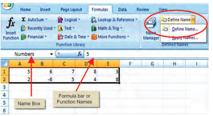
2.     Use the formula bar - This can be found beneath the ribbon. Enter your information directly into the formula bar. By typing the cell number directly into the Name field (found above the Column headings A – Z), you can navigate throughout the worksheet.

3.     Take advantage of Autocomplete. Excel will try to assist you in speeding up your data entry by guessing what you're typing based on the contents of your worksheet.  If the autocorrect option is right for you, just press enter.

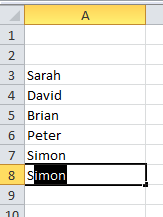
4.     Copy and paste - You may have cells where you may copy and paste data within the same worksheet – saving you time when creating a sheet – or you can copy data to another worksheet within the workbook.

5.     Allow Autofill to handle the heavy lifting. Whether it's text or numbers, autofill choices can finish a series of data. When creating worksheets or entering data, this saves a lot of time.

Copying and moving

You can copy chosen information from the spreadsheet to the Clipboard, which is a temporary storage file in your computer's memory. You can paste any of the objects on the Clipboard into a cell in the same or a different spreadsheet using the Paste feature.

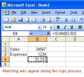
1. Duplicate one or more cells.
2. On the Standard toolbar, click the Copy icon.
3. The replicated cell's border looks like marching ants.

4.     Select the cell where you wish the duplicated data to go. A highlight will be applied to the cell. Click the first cell where you want the copied information to go if you're copying items into multiple cells.

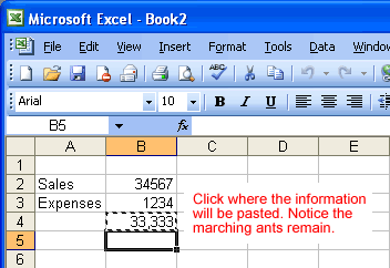
5.     Enter the code with the Enter key. Your data gets transferred to the new location.

If you paste copied cell information into cells that already have data, be careful. Existing data will be overwritten if you do so.

You may paste data into an Excel spreadsheet from a variety of sources, including websites, emails, and other Office products like Word and PowerPoint

Moving data using drag and drop

The drag-and-drop approach is another option for moving data from one cell to another. The cursor is used to point to the information that has to be relocated, and then the cell is dragged to its new location.

●      The cell(s) you want to relocate to a new position should be highlighted and selected.

●      Place the mouse pointer towards one of the selected cell's outside edges (s). The mouse pointer transforms from a large white cross to a thin black cross with arrows on both sides.

●      Keep the mouse pointer on the outer edge of the selected cell and drag the cell(s) to a new location by clicking and holding the left mouse button.

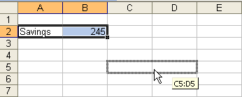
●      To relocate the information to its new location, release the mouse button.

9.5 Handling operators in Formulae

It's possible that you'll wish to change an existing formula at some point. We've provided an inaccurate cell address in our formula in the example below, so we'll need to fix it.

●      Choose the cell that contains the formula you wish to change. In this case, we'll choose cell B3.

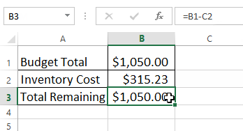
●      To edit the formula, click the formula bar. You may also view and adjust the formula right in the cell by double-clicking it.

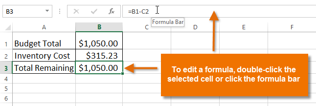
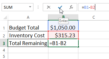
●      Any mentioned cells will be surrounded by a border. We'll update the second section of the formula to refer to cell B2 instead of cell C2 in our example.

●      When you're finished, click the checkmark in the formula bar or press Enter on your keyboard.

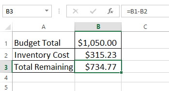
●      The formula will be modified, and the new value in the cell will be displayed.

To avoid mistakenly changing your formula, use the Esc key on your keyboard if you change your mind.

You can hold the Ctrl key and press to see all of the formulas in a spreadsheet (grave accent). The grave accent key is normally found in the keyboard's top-left corner. You can return to the normal view by pressing Ctrl+ again.

9.6 Functions: Mathematical, Logical, statistical, text, financial, Date and Time functions

Mathematical and Statistical function

SUM

When you need to calculate totals for a range of cells or a set of chosen cells on a worksheet, use the SUM function. The totals in row 12 of the Budget Detail worksheet will be calculated using the SUM function. It's worth noting that there are a few different ways to add a function to a worksheet. The following example shows how to add a function to a worksheet by typing it into a cell:

1. To access the worksheet, click the Budget Detail worksheet tab.
2. Cell C12 should be selected.
3. Put an equal sign (=) in the box.
4. SUM is the name of the function.
5. Add an open parenthesis (.) to the end of your sentence.
6. Drag down from cell C3 to cell C11. This inserts the C3:C11 range into the function.
7. Add a closing parenthesis at the end of the sentence.
8. Enter by pressing the ENTER key. The sum for the Monthly Spend column is $1,496 as calculated by the function.

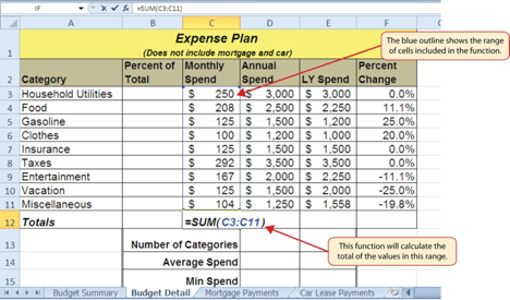
Fig: Adding the SUM Function to the Budget Detail Worksheet

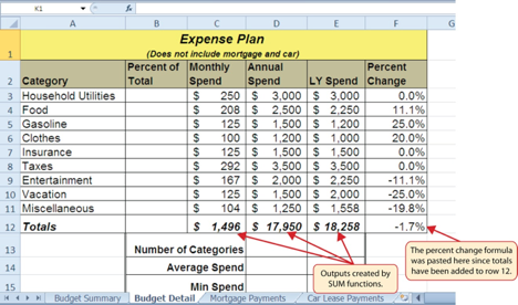
Fig: Results of the SUM Function in the Budget Detail Worksheet

COUNT

When we need to count the number of cells that contain a number, we utilize the count function. Remember, it's all about the numbers! Let's take a look at the function:

COUNT (value1, [value2], …)

So, let's see if we can figure out the answer to our first question: how many things were on sale?

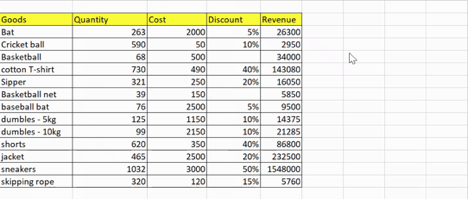
There are 11 discounted items.

AVERAGE

The average is the most prevalent function we employ in our daily lives (or mean). The arithmetic mean of all the cells in a range is returned by the AVERAGE function:

AVERAGE (number1, [number2], …)

However, there is one major disadvantage to employing averages: they are prone to outliers. As a result, in our study, they can portray a very unrealistic picture. Let's figure out how many items were sold on average: dispersed

The average is ~ 365.2 percentile points. We'll be making similar cost estimations as well.

ROUND

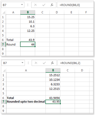
To round an integer to a specific number of digits, use the round function.

Syntax

ROUND(number, number_of_digits)

MOD

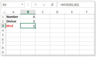
This function is used to calculate the remainder after dividing two numbers.

Syntax

MOD(number,divisor)

CEILING

The Excel Ceiling function rounds a number supplied to the closest multiple of a given number away from zero.

The function's syntax is as follows:

CEILING( number, significance )

The following are the arguments:

Number - This is the number that should be rounded.

Significance - The significance multiple to which the input number should be rounded.

(The arithmetic sign (positive or negative) should be the same as the given number argument.)

Example

The Excel Ceiling function is used in column B of the following spreadsheet to round the positive and negative numbers 22.25 and -22.25 to different significance values.

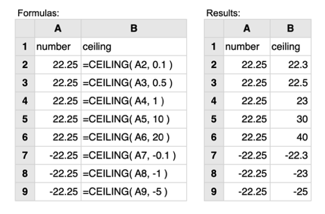
When the number and significance parameters have the same arithmetic sign, the Ceiling function rounds away from zero, as seen in the instances above.

INT

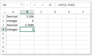
This function transforms a decimal value to an integer that is less than it.

Syntax

INT(decimal number)

ROUNDDOWN

The Rounddown function in Excel reduces a given integer to a defined number of decimal places before rounding it down to zero.

The function's syntax is as follows:

ROUNDDOWN( number, num_digits )

Where the arguments are as follows:

Number - The number that has to be rounded.

Num_digits - To how many decimal places should the input number be rounded.

Note that

●      A positive num digits value indicates the number of digits to the right of the decimal point;

●      a num digits value of 0 indicates rounding to the nearest integer; and a num digits value of -1 indicates rounding to the nearest integer.

●      The number of digits to the left of the decimal point is specified by a negative num digits variable.

Example

The Excel Rounddown function is demonstrated in numerous ways in Column B of the following spreadsheet:

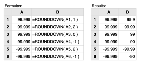
The Rounddown function always rounds down to zero, as shown in the examples above. To put it another way, a positive number gets less positive, whereas a negative number becomes less negative.

ROUNDUP

The Roundup function in Excel takes a number and rounds it up to a specified number of decimal places, away from zero.

The function's syntax is as follows:

ROUNDUP( number, num_digits )

The following are the arguments:

Number - This is the number that should be rounded.

Num_digits - To how many decimal places should the input number be rounded?

Note that

●      A positive num digits value indicates the number of digits to the right of the decimal point;

●      a num digits value of 0 indicates rounding to the nearest integer; and a num digits value of -1 indicates rounding to the nearest integer.

●      The number of digits to the left of the decimal point is specified by a negative num digits variable.

Example

The Excel Roundup function is demonstrated in numerous ways in Column B of the following spreadsheet:

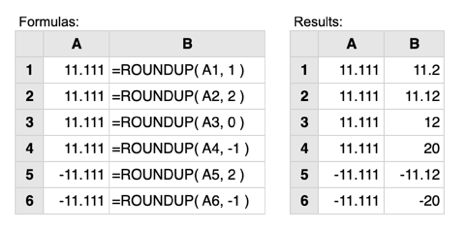
The Roundup function always rounds up, away from zero, as shown in the samples above. A positive number, for example, grows more positive, while a negative number becomes more negative.

FLOOR

The FLOOR function in Excel rounds a number to the nearest multiple of a defined significance to the nearest multiple of zero.

The function's syntax is as follows:

FLOOR( number, significance )

The following are the arguments:

Number - This is the number that should be rounded.

Significance - The significance multiple to which the input number should be rounded.

(The arithmetic sign (positive or negative) should be the same as the given number argument.)

Example

The Excel Floor function is used in column B of the following spreadsheet to round the positive and negative values 26.75 and -26.75 to different multiples of significance.

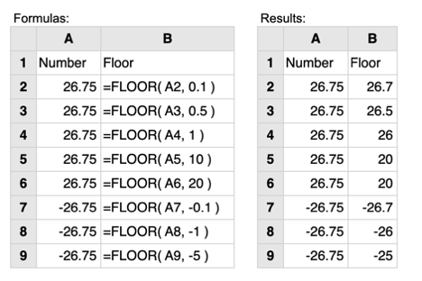
When the number and significance inputs have the same arithmetic sign, the Floor function rounds the given number towards zero, as seen in the examples above.

MAX and MIN

The MAX and MIN functions are the last two statistical functions we'll add to the Budget Detail worksheet. The highest and lowest values in a set of cells are identified using these functions. The methods below will show you how to add these features to the Budget Detail worksheet:

1. In the Budget Detail spreadsheet, click cell D15.
2. Put an equal sign (=) in the box.
3. Fill in the blanks with the word MIN.
4. Add an open parenthesis (.) to the end of your sentence.
5. The range D3:D11 should be highlighted.
6. If you type a closing parenthesis and press the ENTER key, Excel will close the function for you. The lowest figure in the Annual Spend column is $1,200, which is the result of the MIN function.
7. D16 is the cell to click.
8. Put an equal sign (=) in the box.
9. Fill in the blanks with the word MAX.
10. Add an open parenthesis (.) to the end of your sentence.
11. The range D3:D11 should be highlighted.
12. If you type a closing parenthesis and press the ENTER key, Excel will close the function for you. The MAX function returns $3,500 as a result. In the Annual Spend column, this is the highest figure.

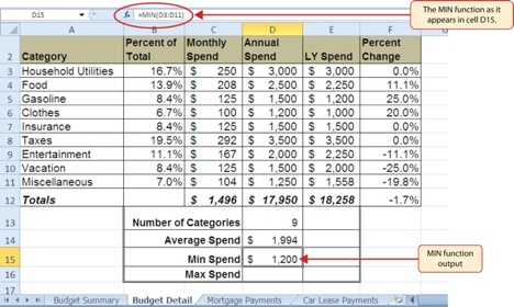
Fig: MIN Function Added to the Budget Detail Worksheet

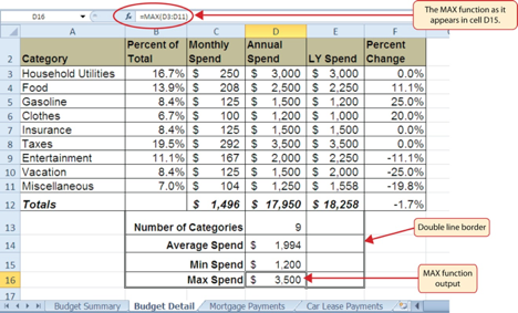
Fig: MAX Function Added to the Budget Detail Worksheet

SQRT

The Sqrt function in Excel determines the positive square root of a given value.

The function's syntax is as follows:

SQRT( number )

Where the number input is the numeric value whose square root you want to find.

The Sqrt function returns the #NUM! error if the provided number is negative.

Example

Three simple examples of the Excel Sqrt function are shown in the spreadsheet below.

Logical function

To work with logical values, Microsoft Excel includes four logical functions. AND, OR, XOR, and NOT are the functions. When you wish to do many comparisons in your calculation or test multiple conditions instead of just one, you use these functions. When their parameters are evaluated, Excel logical functions return TRUE or FALSE, just like logical operators.

To assist you find the correct formula for a certain assignment, the table below provides a brief overview of what each logical function accomplishes.

Text function

Within an Excel spreadsheet, the TEXT Function is used to transform integers to text. The function essentially converts a numeric number to a text string. TEXT is available in all Excel versions.

The syntax of this function translates a numeric value to text in a specified number format:

Text(Value, format_text)

Where,

Value - A numeric value, a formula that evaluates to a numeric value, or a reference to a cell that has a numeric value are all examples of value.

Format_text - is a number format that takes the form of a text string surrounded by quotation marks. By selecting Number, Date, Time, Currency, or Custom from the Category box of the Number tab in the Format Cells dialog box, and then viewing the formats provided, we may see a variety of numeric formats.

When is the Excel TEXT Function required?

The TEXT function is used in the following situations:

●      When we need dates to be displayed in a specific format.

●      When we want numbers to be displayed in a specific format or in a more readable way.

●      When we want to merge text or characters with numbers.

Example

I need to convert the following data to the “d mmmm, yyyy” format. When we use the text function, the following is the result:

Financial functions

FV (future value)

Use the following formula to calculate the future value of a certain investment with a constant interest rate and monthly payments:

FV (Rate, Nper, [Pmt], PV, [Type])

●      Rate = It is the interest rate/period

●      Nper = Number of periods

●      [Pmt] = Payment/period

●      PV = Present Value

●      [Type] = When the payment is made (if nothing is mentioned, it’s assumed that the payment has been made at the end of the period)

Example

In 2016, A made a $100 investment. The payment was made on a yearly basis. The annual interest rate is 10%. What will the FV be in 2019?

We'll write the equation in Excel as follows:

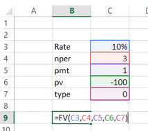
= FV (10%, 3, 1, – 100)

= US $129.79

PV (present value)

It's easier to figure out PV if you know how to calculate FV. Here's how it works:

PV = (Rate, Nper, [Pmt], FV, [Type])

●      Rate = It is the interest rate/period

●      Nper = Number of periods

●      [Pmt] = Payment/period

●      FV = Future Value

●      [Type] = When the payment is made (if nothing else is specified, the payment is presumed to be made at the end of the period)

Example

In 2019, the value of a $100 investment in the United States. The payment was made on a yearly basis. The annual interest rate is 10%. What would be the current PV?

We'll write the equation in Excel as follows:

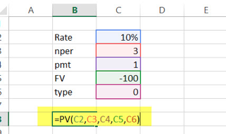
= PV (10%, 3, 1, – 100)

= US $72.64

PMT

In Excel, PMT stands for periodic payments required to pay off a debt over a set length of time at a fixed interest rate. Let's have a look at how to do it in Excel.

PMT = (Rate, Nper, PV, [FV], [Type])

●      Rate = It is the interest rate/period

●      Nper = Number of periods

●      PV = Present Value

●      [FV] = An optional argument that concerns the loan's future value (if nothing is mentioned, FV is considered as “0”)

●      [Type] = When the payment is made (if nothing else is specified, the payment is presumed to be made at the end of the period)

Example

The $1000 must be paid in full within three years. The interest rate is 10% p.a., and the payment must be made once a year. Find out what the PMT is.

In Excel, we'll compute it as follows:

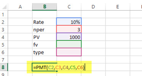
= PMT (10%, 3, 1000)

= – 402.11

PPMT

It's a different type of PMT. The sole distinction is that PPMT uses a constant interest rate and periodic payments to calculate payments on principle. Here's how to figure out your PPMT.

PPMT = (Rate, Per, Nper, PV, [FV], [Type])

●      Rate = It is the interest rate/period

●      Per = The period for which the principal is to be calculated

●      Nper = Number of periods

●      PV = Present Value

●      [FV] = An optional input that refers to a loan's future value (if none is given, FV is assumed to be "0")

●      [Type] = When the payment is made (if nothing else is specified, the payment is presumed to be made at the end of the period)

Example

The $1000 must be paid in full within three years. The interest rate is 10% p.a., and the payment must be made once a year. In the first and second years, find out what the PPMT is.

In Excel, we'll compute it as follows:

1st year

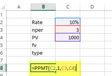
=PPMT (10%, 1, 3, 1000)

= US $-302.11

2nd year

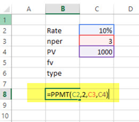
=PPMT (10%, 2, 3, 1000)

= US $-332.33

IPMT

Consider a loan with an annual interest rate of 5%, a 2-year duration and a present value (amount borrowed) of $20,000.

The interest portion of the payment is calculated using Excel's IPMT function. The payment number is specified by the second argument.

The interest portion of the 5th payment is calculated using the IPMT function.

NPER

It simply refers to the number of repayment periods required to repay the loan.

NPER = (Rate, PMT, PV, [FV], [Type])

●      Rate = It is the interest rate/period

●      PMT = Amount paid per period

●      PV = Present Value

●      [FV] = An optional argument which is about the future value of a loan (if nothing is mentioned, FV is considered as “0”)

●      [Type] = When the payment is made (if nothing is mentioned, it’s assumed that the payment has been made at the end of the period.

Example

For a loan of $1000, a yearly payment of $200 is made. The interest rate is 10% p.a., and the payment must be made once a year. Find out what the NPER is.

NPER must be calculated in the following way:

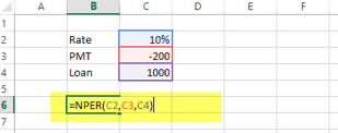
= NPER (10%, -200, 1000)

= 7.27 years

RATE

We can determine the interest rate required to pay off the debt in full for a particular period of time using the RATE function in Excel. Let's have a look at how to use the RATE finance function in Excel to calculate rates.

RATE = (NPER, PMT, PV, [FV], [Type], [Guess])

●      Nper = Number of periods

●      PMT = Amount paid per period

●      PV = Present Value

●      [FV] = An optional argument which is about the future value of a loan (if nothing is mentioned, FV is considered as “0”)

●      [Type] = When the payment is made (if nothing is mentioned, it’s assumed that the payment has been made at the end of the period)

●      [Guess] = An assumption of what you think RATE should be

Example

The payment for a loan of US $1000 over 6 years is $200 per year, and the payment must be made on a yearly basis. Find out what the RATE is.

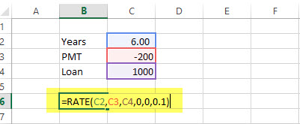
= RATE (6, -200, 1000, 0.1)

= 5%

Date and Time functions

DATE()

The DATE function returns a sequential serial number that corresponds to a specific date.

The result is presented as a date instead of a number if the cell format was General before the function was entered. Adjust the cell format to see the serial number or to change the date formatting.

Syntax

DATE(year, months, day)

Example - The example below shows the serial data or the date derived by using year as 2004 and month as 12 and day as 22.

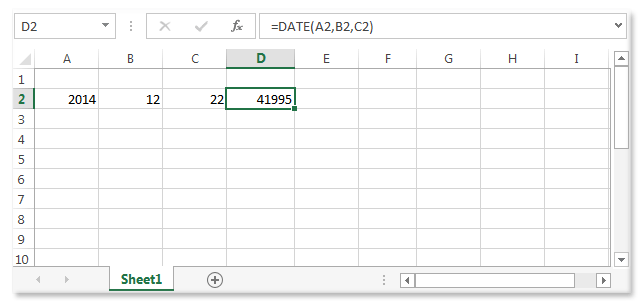
TIME () function

This function is used to get the decimal value for a specific period. If the cell format was General before the function, the result is formatted as a date.

TIME returns a decimal number ranging from 0 (zero) to 0.99988426, which represents times from 0:00:00 (12:00:00 AM) to 23:59:59. (11:59:59 P.M.).

Syntax

TIME (hour, minute, second)

Example - The example below returns the decimal part of a day, for the time specified in row 4 (14 hours, 10, minutes, 15 seconds)

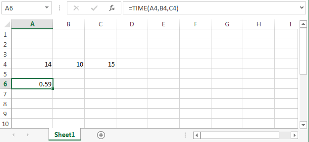
TODAY()

TODAY () in the blank worksheet, this is the function for today's date.

TODAY — The current date's serial number is returned. The serial number is a date-time code that Excel uses to calculate dates and times. Fractions of a day are used to denote times. Serial number 1 is assigned by default on January 1, 1900. As a result, the serial number for January 1, 2009 is 39814. (because it is 39814 days after January 1, 1900).

9.7 Using Function Wizard

Through submenus and categories, the function wizard opens all of Excel's functions. To use the Function Wizard, go to the Insert menu and select Function, or go to the Standard toolbar and select the Function Wizard button "fx." Click on each Function category with your mouse to explore the Functions. The "Average" Function is used as an example in the following example.

The Function Wizard can assist you in locating a function and providing step-by-step instructions on how to utilize it. Click the Insert Function button on the Formula Bar or the Insert Function button on the Formulas tab to open the Function Wizard.

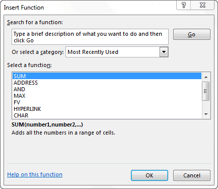
Type a description in the Search for a Function section and then click Go to find the function you're looking for. In the Select a Function Field, Excel will show you all of the functions that match your criteria. Then click OK after selecting the desired function. Excel will provide a dialog box tailored to the function you selected.

Alternatively, specify the category your function belongs to using the Or Select a Category Field. In the Select a Function Field, Excel will show you all of the functions in that category. Then click OK after selecting the desired function. Excel will provide a dialog box tailored to the function you selected.

There is a separate dialog box for each function. The Function Specific dialog box is how I refer to it. Each of the function's arguments is listed in the Function Specific dialog box. Type the appropriate value in each field, or select a range by clicking in the field and dragging. Click OK once you've entered all of your arguments. Excel will enter the function in your formula.

You can access the Function Wizard at any moment by clicking the Insert Function button when typing a formula into a cell or into the Formula Bar. Excel will send you immediately to the Function Specific dialog box if you type the function name or choose the function from the AutoComplete List, then click the Insert Function button.

Use the function wizard

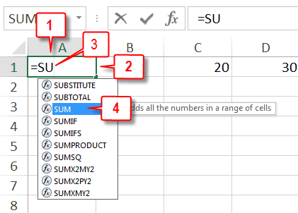
1. Go to the cell where you wish the formula's results to appear.
2. Type in the cell or in the Formula Bar to get started.
3. Begin typing the function name when you need to utilize it.
4. Click the function name in the AutoComplete list when you see it.

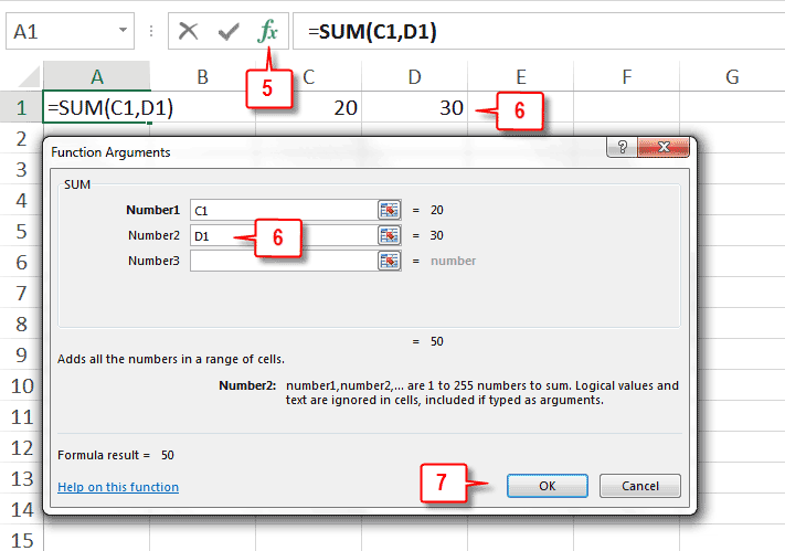
5.     Select Insert Function from the drop-down menu. The function you selected opens in a dialog window.

6.     Put your points forward. When you wish to refer to a cell, simply click it. When you want to refer to a range, select it by clicking and dragging.

7.     Click OK when you've finished your function.

8.     Continue to type your formula in.

9.     When you've finished your entry, press Enter or click the Enter button on the Formula Bar.

9.8 Formatting a Worksheet: Formatting Cells changing data alignment, changing font, adding borders and colors, Printing worksheets

Select the cell or cells you want to align first. Text in a single cell, a range of cells, a row or rows, a column or columns, or the entire worksheet can be aligned. (To select all cells, press Ctrl+A.)

1. Choose the cells you'd like to align.
2. Select a horizontal alignment option in the Alignment group on the Home tab:

Align left  center   Align right

3.     Select a vertical alignment option in the Alignment group on the Home tab:

Top align  Middle align  Bottom align

You can adjust the font angle or change the text alignment to alter the appearance of data in a cell.

Change the orientation of text in a cell

1. Choose a cell, a row, a column, or a range of cells.
2. Select Home > Orientation  , and then select an option.

You can align text vertically or rotate it up, down, clockwise, or counterclockwise:

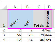
Rotate text to a precise angle

1. Select a cell, row, column, or a range.
2. Select Home > Orientation    > Format Cell Alignment.
3. Under Orientation on the right side, in the Degrees box, use the up or down arrow to set the exact number of degrees that you want to rotate the selected cell text.

Positive numbers rotate the text upward. Negative numbers rotate the text downward.

Changing font

Excel uses the Calibri font style in size11 when you input data in a spreadsheet, but if you prefer a different font style or size, here's how to alter them:

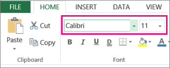
1. Choose the cell or cell range in which you want to format the text or number.
2. Select a different font by clicking the arrow next to Font.

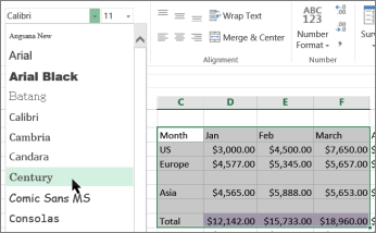
1. To alter the font size, select the desired size by clicking the arrow adjacent to the default Font Size.

We've modified the font style to Century and the size to 9 in the sample below.

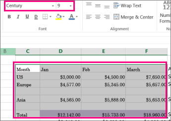
Data entered in cells outside of the newly formatted cell range will be shown in the default style and size, and you'll have to repeat the formatting procedures. Before entering data, you can also choose blank cells and apply formatting.

Adding border and colors

You may simply add a border around cells or ranges of cells by utilizing predefined border styles. You can construct a custom border if the standard cell boundaries do not match your needs.

Select the cell or set of cells on a worksheet for which you want to add a border, change the border style, or delete a border.

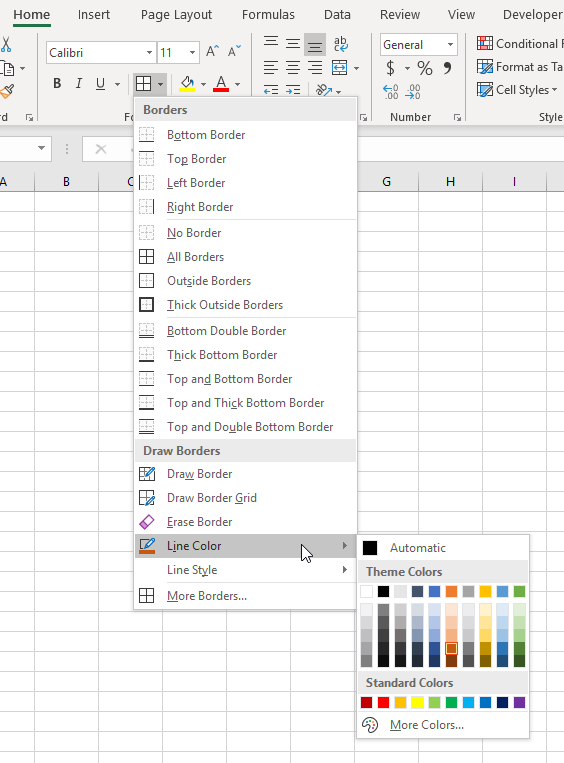
Do one of the following on the Home tab, in the Font group:

●      Pick the arrow adjacent to the Borders , then click a border style to apply a new or different border style.

●      Click the arrow next to the Borders , then click the No Border to remove cell borders.

The Borders button shows the most recent border style that has been used. To apply that style, click the Borders button (not the arrow).

When you apply a border to a cell, it is applied to any adjacent cells that share a bordered cell boundary. When you use a box border to surround the range B1:C5, for example, the cells D1:D5 get a left border.

When two types of borders are applied to a common cell boundary, the most recently applied border is shown.

A single block of cells is prepared from a selected range of cells. When you apply a right border to the range of cells B1:C5, only the right edge of the cells C1:C5 are bordered.

You can use an inner border to print the same border on cells separated by a page break, but the border will only appear on one page. This manner, you can print a border at the bottom of one page's last row and the same border at the top of the next page's first row. Perform the following actions:

●      On both sides of the page break, choose the rows.

●      More Borders can be accessed by clicking the arrow next to the Borders Button image.

●      Click the Inside button Button image under Presets.

●      Remove the vertical border in the preview diagram by clicking it under Border.

Colors

Excel allows you to apply borders to your cells, as you surely already know. This is useful for separating distinct types of information within the same data table, as well as simply improving the appearance of your data.

However, black borders aren't the only option. By following these instructions, you can change the color of your borders:

1. Change the border colors of the cells you want to change.
2. Make sure the ribbon's Home tab is visible.
3. Click the down-arrow next to the Borders tool in the Font group. You'll see a list of cell borders that you can use.
4. At the bottom of the list, select the More Borders option. The Border tab of the Format Cells dialog box appears in Excel.

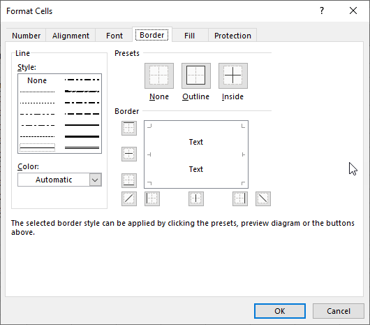
5.     Select a color for the borders from the Color drop-down list.

6.     Set the cell's borders as you normally would using the controls in the dialog box.

7.     Click the OK button.

You can provide a distinct border type and color for each side of a cell, just like you can specify a different border type and color for each side of a cell. Simply choose the color you wish to use before clicking on the side of the cell where you want it to appear.

You can also utilize the border drawing tools Excel provides to modify the border color. Simply click the down-arrow next to the Borders tool on the Home tab of the ribbon (in the Font group). Excel displays a whole bunch of choices for applying borders.

Printing worksheet

You can print complete or partial worksheets and workbooks one at a time or in batches. You can also print simply the Excel table if the data you wish to publish is in a Microsoft Excel table.

Instead of printing to a printer, you can save a workbook as a file. This is important if you need to print the workbook on a printer that isn't the same as the one you used to print it the first time.

Print one or several worksheets

1. Choose which worksheets you wish to print.
2. Press CTRL+P or go to File > Print.
3. Before you click the Print button, you can either alter the settings or click the Print button.

Print one or several workbooks

You must keep all workbook files in the same folder if you wish to print them.

●      Click File > Open.

●      CTRL-click the name of each worksheet you want to print, then click Print.

Print all or part of a worksheet

●      Select the range of data you want to print by clicking the worksheet and then selecting the range of data you want to print.

●      Then, under File, select Print.

●      Select the appropriate option by clicking the arrow next to Print Active Sheets under Settings.

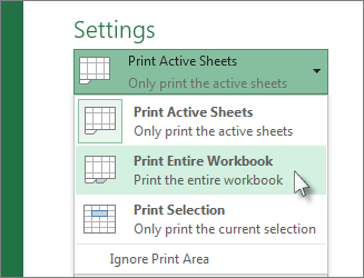
●      Click print.

9.9 Changing date, number, character or currency format

In a spreadsheet, to format or change the format of numbers, dates, or currencies:

●      Open a Google Sheets spreadsheet on your PC.

●      Choose the range of cells you want to format or change.

●      Then select Number from the Format drop-down menu.

●      Choose a format for the cells in the range.

Custom formatting of numbers, dates, and currencies

Custom formatting is available for currencies, dates, and numbers. You may find the format that works for your spreadsheet in the text fields accessible in the formatting selections for each of them. If you can't find what you're searching for, you may now use the menus to design your own unique layout.

Date

To add a custom date or time format to your spreadsheet, follow these steps:

1. Open a Google Sheets spreadsheet on your PC.
2. Make a note of the data you want to format.
3. Select Format, Number, and More Formats from the drop-down menu.
4. More date and time formats can be found by clicking the link.
5. To choose a format, type it into the menu text box. In the text area, you can also provide your own unique date or time format.
6. Apply the changes.

By default, the time and date options that appear are based on the location of your spreadsheet.

Click the down arrow in the right corner of the menu text box and select an additional value if you want to add more detailed time or date data to your formatting, such as the hour or minute. By clicking on the arrows in the value and selecting an option, you can change the specific formatting for these values. To remove a value from your formatting, right-click it and choose Delete.

Number

To add a custom currency format to your spreadsheet, follow these steps:

1. Open a Google Sheets spreadsheet on your PC.
2. Make a note of the data you want to format.
3. Select Format, Number, and More Formats from the drop-down menu.
4. More currencies can be found by clicking on the link.
5. To choose a format, type it into the menu text box. In the text area, you can also specify your own unique currency format.
6. Apply the changes.

By selecting an option from the drop-down menu in the right corner of the input box, you can adjust a few aspects about the currency (for example, how many decimal places to show).

Currency and Character

To add a custom number format to your spreadsheet, follow these steps:

1. Open a Google Sheets spreadsheet on your PC.
2. Make a note of the data you want to format.
3. Select Format, Number, and More Formats from the drop-down menu.
4. Select Custom number format from the dropdown menu.
5. To choose a format, type it into the menu text box. In the text area, you can also provide your own custom number format.
6. Apply the changes.

When developing a custom format, keep in mind that it can have up to four components, each separated by a semicolon: positive; negative; zero; non-numeric. There are various financial formats that can be used.

Colors can be used in the formatting to distinguish positive and negative integers, for example, by putting a color in brackets (for example, [Red]) anywhere inside the relevant area of the style. In English, color formatting is required. The following colors can be used:

The following is a list of commonly used syntax characters for creating a bespoke number format:

9.10 Charts and Graphs – Creating, Previewing, Modifying Charts

After you've entered your data and selected a cell range, you'll need to choose a chart type to display it. We'll use the data we used to make a clustered column chart in this example.

Step 1: Select Chart Type

Click the Insert tab on the top banner once your data has been highlighted in the Workbook. A section with many chart options is located about halfway down the toolbar. Recommended Charts are based on popularity, but you can choose a different template by clicking any of the dropdown choices.

Step 2: Create Your Chart

1. Select Clustered Column from the Column Chart icon on the Insert tab.

1. Excel will generate a clustered chart column based on the data you've chosen. The chart will show in the workbook's middle.
2. To give your chart a name, double-click the Chart Title text and input a title. This graph will be referred to as "Product Profit 2013 - 2017."

Step 3: Add Chart Elements

By adding chart elements to a graph or chart, you can improve it by clarifying data or adding context. By using the Add Chart Element dropdown menu in the top left corner, you may choose a chart element (beneath the Home tab).

Step 4: Adjust Quick Layout

1. Quick Layout is the toolbar's second dropdown menu, and it allows you to quickly change the layout of components in your chart (titles, legend, clusters etc.).

2.     There are 11 quick layout alternatives to choose from. Hover your cursor over the various options for a description, then select the one you want to use.

Step 5: Change Colors

Change Colors is the next dropdown menu in the toolbar. Choose the color palette that best suits your demands (they could be aesthetic or to match the colors and design of your brand).

Step 6: Change Style

There are 14 chart styles available for cluster column charts. The chart will be displayed in Style 1 by default, but you can alter it to any of the other styles. To see more possibilities, click the arrow to the right of the image bar.

Step 7: Switch Row/Column

To flip the axis, click the Switch Row/Column button in the toolbar. Note that flipping axes for each chart, for example, if you have more than two variables, is not always straightforward.

Switching the row and column in this example switches the product and year (profit remains on the y-axis). The graph is now organized by product (rather than by year), and the color-coded legend corresponds to the year (not product). To avoid any misunderstanding, go to the legend and change the Series to Years titles.

Step 8: Select Data

1. To adjust the range of your data, click the Select Data icon on the toolbar.

2.     A door will swing open. Click the OK button after you've typed in the cell range you desire. This updated data range will be reflected in the chart automatically.

Step 9: Change Chart Type

1. Change the chart type from the dropdown menu.

2.     You can modify the chart type to any of Excel's nine chart types from here. Of course, double-check that your data is suitable for the chart type you've chosen.

3.     By clicking Save as Template..., you may easily save your chart as a template.

4.     You'll be presented with a dialogue window where you may give your template a name. For simple organizing, Excel will automatically create a folder for your templates. To save your work, click the blue Save button.

Step 10: Move chart

1. On the far right of the toolbar, click the Move Chart symbol.

2.     You'll see a dialogue window where you can pick where to put your chart. You may either use this chart to build a new sheet (New sheet) or use it as an object in another sheet (Object in). To continue, press the blue OK button.

Step 11: Change formatting

1. You can modify the colors, size, shape, fill, and alignment of all elements and text in the chart, as well as insert shapes, using the Format tab. To make a chart that fits your company's brand, go to the Format tab and use the shortcuts available (colors, images, etc.).

2.     Select the chart element you want to alter from the dropdown menu on the upper left side of the toolbar.

Step 12: Delete a chart

Simply choose a chart and press the Delete key on your keyboard to delete it.

Previewing

You can see a preview of how the data will appear on the printed if you pick one or more sheets and then click File > Print.

1. Choose the worksheet(s) you'd like to see a preview of.
2. To access the Preview window and printing options, go to File, then Print.

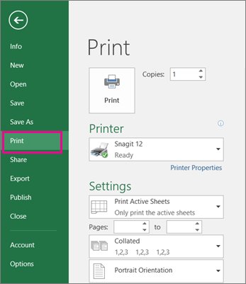
Keyboard shortcut You can also press Ctrl+F2.

Some more points

●      Click the arrows for Next Page and Previous Page at the bottom of the Print See window—or type the page number—to preview the next and previous pages.

●      Click any of the arrows in the upper-left corner of the Print Preview window to exit Print Preview and return to your workbook.

●      Click the Show Margins button in the lower right corner of the Print Preview window to see page margins.

●      To alter the margins, drag them to the desired height and width. Drag the handles at the top and bottom of the print preview page to modify the column widths. Set page margins before printing a worksheet for additional information on page margins.

Modifying chart

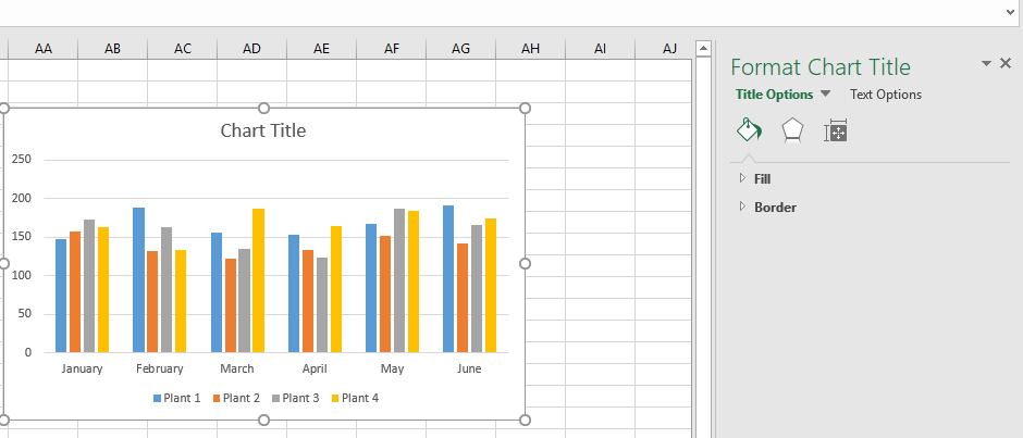
Once the chart is in Excel, you may change its appearance and location in a variety of ways. A few options are listed here, but there are many more! To access Chart Tools in any situation, you must first pick the chart.

●      To add any labels (such as the title or axis), click Add Chart Element in the Chart Layouts group on the Design ribbon and choose the desired label.

●      Use the Chart Tools Design ribbon to alter the chart type, data, or location.

You can choose an element on the chart (for example, a series) and then choose the Format Selection icon in the Current Selection group from the Chart Tools Format ribbon.

9.11 Integrating word processor, spreadsheets, web pages

Word processing is one of the most common computer applications today. A day in a modern office or university would be difficult to imagine without coming into contact with a word processing program. The majority of people have had some experience with word processing. We'll go over the concept in depth so you'll be familiar with the various levels of word processing software applications, the types of tools these programs provide, and the types of problems that are best solved with this type of program.

How Word Processors Work

Consider some of the drawbacks of typewriters to better understand the benefits of word processing programs. When we use a typewriter to create a document, the keys and the paper are in direct contact. When you press a key on the keyboard, it makes a physical impact on the paper, and the document is changed. If you catch a mistake early enough, you can use correction tape or white-out to correct it. It is much more difficult to correct a mistake that is more than one character long. You must totally retype the page if you want to add a word, relocate a paragraph, or adjust the margins. This may necessitate adjustments to other pages as well.

Word processing software is a type of program that focuses on text handling. The computer accomplishes this by giving a numeric code to each letter of the alphabet and each other character on the keyboard. These numeric codes are converted to machine language and saved in the computer's memory. Because the data is stored in memory, it is incredibly simple to alter and manipulate. This is the key to word processing's success.

Example

Memory information may be moved fast and easily. What happens in the computer when we wish to edit a word in a document is as follows:

Assume Darlene's résumé begins with the following phrase:

REUME

Clearly, she has misplaced a letter. If she had used a typewriter, the page would have been thrown away, and she would have had to start over. Darlene may change the memory containing codes for the word "REUME" and add the "S" because this is a word processor. When she makes an attempt, the following things occur:

She positions her cursor where she wants the S to appear in the text. The "cursor" is a distinctive indicator on the screen that indicates where the computer is now focused in the page. Darlene wants to add a S between the E and the U in this situation. Because her word processor won't allow her put the cursor between two letters (though others will), she chooses the letter U.

Darlene is instructing the program to go around in memory by moving the pointer. She tells the program to point to the corresponding spot in the computer's memory when she places her cursor on the U on the screen. The computer's attention is now drawn to the memory cell containing the code for the character "U."

She double-checks that she's in insert mode (more on that later) before typing the letter "S."

When Darlene does this, the computer moves all of the letters one memory cell to the right and puts the S code where it belongs.

Integrated package

These software programs are frequently included when a customer purchases a new computer system. An integrated package is a large program that includes a word processor, spreadsheet, database tool, and other software programs all in one place. (Don't worry if you've never heard of a spreadsheet or a database.) We'll be there in no time!) An integrated application package is similar to a software "Swiss army knife."

An integrated package's benefits stem from the fact that all of the applications are part of the same program and were produced by the same business. It should be relatively simple to combine the components of an integrated package. Because some programs are smaller, older versions of larger programs, they may be easier to use. They should all have the same overall menu structure and commands because they were likely written together. (For example, in all programs, the command to save a file would be the same set of keystrokes.) Integrated packages are frequently created with non-technical users in mind. This may make them more user-friendly than more powerful programs. An integrated package's word processor is likely to be more powerful than a standard text editor.

Because integrated packages are frequently pre-installed on new computers, they may not cost you any more than the computer's initial purchase price. An integrated package's word processor will almost probably have functionality that you won't find in conventional text editors.

There are various drawbacks to using integrated packages. Programs have grown more and more standard as graphical user interfaces and modern operating systems have become more common, even if they were built by different organizations. For example, almost every Windows software utilizes Alt-F-S to save.

Additionally, similar to the Swiss army knife analogy, the programmers had to make some concessions in order to put all of the apps into one software. Although a Swiss army knife has a saw, wouldn't you rather use a real saw to cut down a tree? An integrated package's programs are frequently stripped-down versions of the company's high-end software. They have fewer features and are likely to be less welcoming. Although they can usually read and write ASCII, word processing tools that are part of integrated packages usually have their own specific coding for storing text information.

Common Integrated Packages:

●      Microsoft Works

●      Lotus Works

●      Claris Works

Spreadsheets

A spreadsheet is a file with rows and columns of cells that can be used to organize, calculate, and sort data. Numeric values, text, formulas, references, and functions can all be found in a spreadsheet.

Spreadsheets are grid-based files that are used to maintain or conduct calculations on personal or business data. It is featured in MS Office and Office 365, and it allows users to generate spreadsheets. MS Office is an on-premise application, whereas Office 365 is a cloud-based solution. There are more than 400 functions and features, including pivot, coloring, graph, chart, conditional formatting, and many others, making it the greatest choice for users.

The term "workbook" in Excel refers to a "spreadsheet." This phrase is used by Microsoft Excel to stress the fact that a single workbook can contain several worksheets, each with its own data grid, chart, or graph.

The most typical reason for using spreadsheets is to organize and store data such as revenue, payroll, and accounting data. Spreadsheets allow the user to perform calculations and create graphs and charts using the data.

In a spreadsheet, the rows have numeric names (1, 2, 3, etc.) and the columns have alphabetic names (a, b, c, etc.), therefore cell names consist of a letter and a number that indicate their location in the grid.

Selection of rows

Row 3 is selected in the illustration above. By clicking on the number 3 in front of the row, you can do so.

Selection of column

Column B is selected in the illustration above. By clicking on the letter B above the column, you can do so.

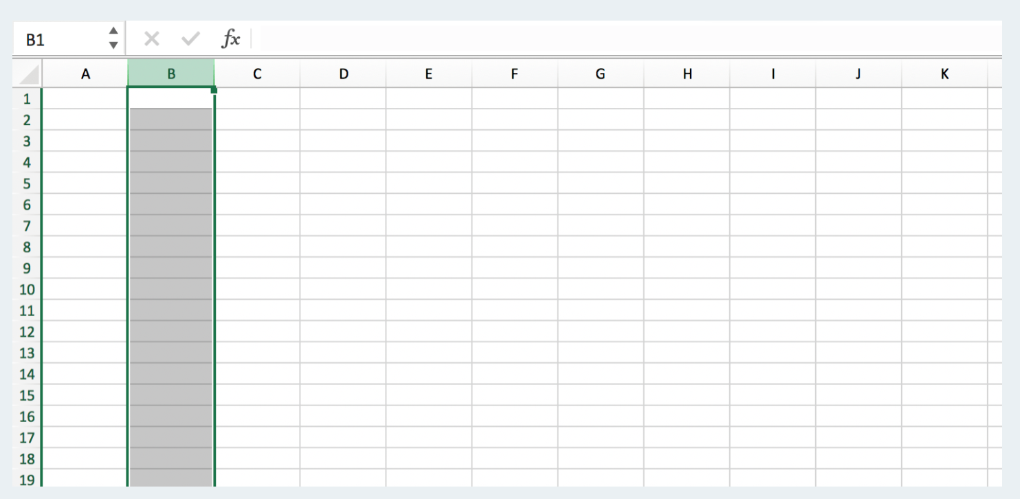
Selection of cell

Cell B3 is picked in the image above. By clicking on the cell, you can do so.

Worksheet

One or more worksheets can be found in a spreadsheet (tabs). By pressing the ‘+' on the right side of the existing worksheet tab, you can add further worksheets (s).

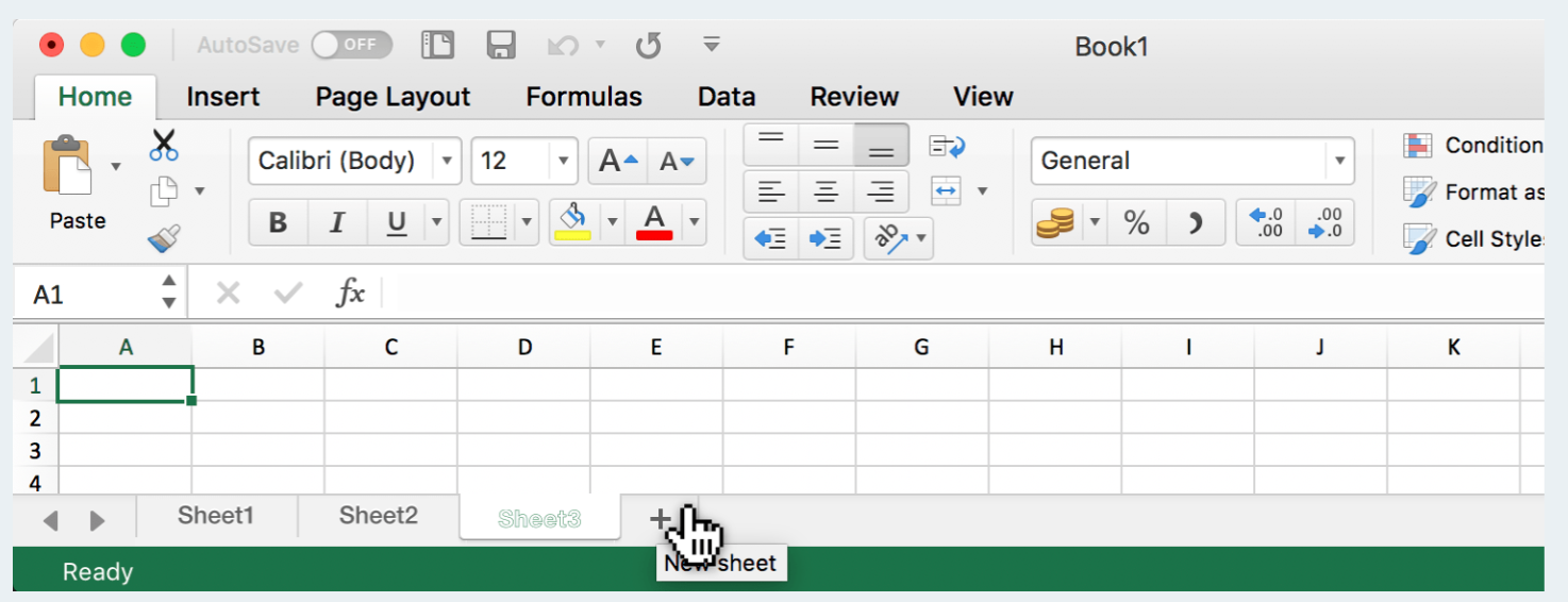
Worksheet 3 is selected in the image above. A new worksheet will be added to the spreadsheet by clicking the plus sign.

Web pages

If you get data from the Web (and who doesn't these days? ), you probably print the page and then manually re-enter the information. Ouch! You should never have to re-enter data if you don't have to, and you don't have to in this situation. Instead, open the Web page directly in Excel by typing:

●      From the File menu, select Open. In Excel 2007, the Open command is found on the Office menu.

●      In the File Name text box, type the URL, including the http://. A "connected to server" notice will most likely appear in Excel. That's alright; don't be concerned.

●      From the Files Of Type control, select Web Pages And Web Archives (*.htm; *.html; *.mht; *.mhtml). All Web Pages is the file type in Excel 2007. (*.htm; *.html; *.mht; *.mhtml).

●      Click the Open button.

The transferred data from the Web page is really entered into the current sheet, and you can alter it just like any other data. Go ahead and click one of the hyperlinks! They should operate properly as long as you're connected to the Internet.

However, the final Excel sheet will not resemble the Web page. It's a straightforward data transmission, and Excel isn't a browser. This tool, on the other hand, is a quick and simple approach to obtain the raw data you require onto a sheet. Delete any unnecessary visuals, then duplicate or transpose data blocks to arrange the elements exactly how you want them. The data can even be shared with other Office programs.

9.12 Pivot table

A pivot table is a data summarizing tool used in the context of data management. To summarize, sort, reorganize, group, check, aggregate, or standard record held in a database, pivot tables are used. It allows users to convert columns to rows and rows to segments. It allows for grouping based on any data column. When we need to summarize and analyze a large amount of data, pivot tables are the best option.

Starting with a blank Pivot Table

●      Open the GL Pivot Table Data.xlsx spreadsheet. A query is included in the spreadsheet, which includes FY11 costs from the Economic Data Warehouse.

●      Place our cursor in any cell in the data.

●      Open the insert Tab from the ribbon.

●      To access a list of options, click the Pivot Table down arrow.

1. Choose the cells from which you wish to make a PivotTable.
2. Select Insert > PivotTable.

3.     Select the data you want to study under Choose the data you want to analyze. Choose a table or a range of tables.

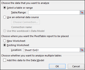
4.     Verify the cell range in Table/Range.

5.     Select New worksheet to place the PivotTable report in a new worksheet or Existing worksheet to place the PivotTable in an existing worksheet, and then select the location you want the PivotTable to appear under Choose where you want the PivotTable report to appear.

6.     Choose OK.

Building out your PivotTable

1. Select the field name checkbox in the PivotTables Fields window to add a field to your PivotTable.

(Non-numeric fields are moved to Rows, date and time hierarchies are moved to Columns, and numeric fields are moved to Values.)

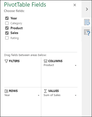
2.     Drag a field to the target region to shift it from one location to another.

9.13 Goal seek

The Goal Seek Excel function (also known as What-if-Analysis) is a method of determining a desired output by altering an underlying assumption. The function effectively back-solves the problem by trial and error, entering in guesses until it finds the answer. If the revenue formula is the number of units sold multiplied by the selling price, Goal Seek may calculate how many units must be sold to generate $1 million in revenue if the selling price is known. The function comes in handy when it comes to sensitivity analysis in financial modeling.

If you know the formula result you want, utilize Excel's Goal Seek feature to discover the input value that delivers it.

Example

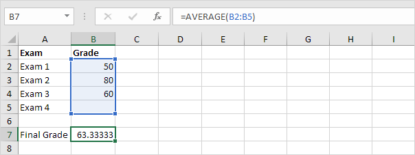
Find the grade on the fourth exam that results in a final grade of 70 using Goal Seek in Excel.

●      The final grade is calculated using the algorithm in cell B7.

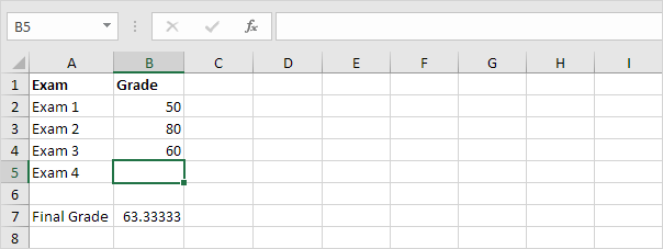
●      The input cell is cell B5, which contains the grade from the fourth exam.

●      Click What-If Analysis in the Forecast group on the Data tab.

The dialog window for Goal Seek appears.

●      B7 is the cell to be selected.

●      Type 70 in the box labeled "To value."

●      Select cell B5 from the 'By changing cell' box.

●      Click ok.

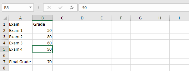
Result. A final grade of 70 is obtained by receiving a 90 on the fourth exam.

9.14 Data filter and scenario manager

Scenario manager

When you have several variables and want to observe how changing these variables affects the final outcome, Scenario Manager in Excel is a good tool to use.

Assume you have the following dataset and wish to determine the profit value:

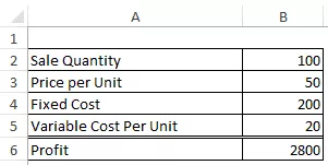
The profit value is determined by three factors: the number of units sold, the price per unit, and the variable cost per unit. Here's the calculation I used to figure out the profit:

=B2*B3-B4-B5*B2

The goal is to see how the final result changes as the dependent variables are changed.

You can create a one-variable or two-variable data table, as illustrated in the first two articles of this series, if just one or two variables are changing. However, scenario manager is the way to go if you have three or more variables that can change.

Setting up scenario manager

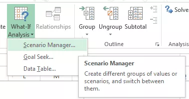
●      Go to Data Tab –> Data Tools –> What-If Analysis –> Scenario Manager.

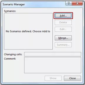
●      In the Scenario Manager dialogue box, click on Add.

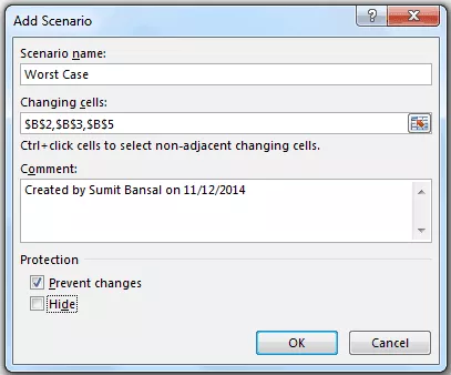
●      In the Add Scenario dialogue box, fill in the following details:

○      Scenario name: Worst Case

○      Changing cells: $B$2,$B$3,$B$5 (you can also select it by pressing the CONTROL button and using mouse left-click).

○      Comment: Any comment you wish you add. You can also leave this blank.

●      Click OK. This opens the Scenario Values dialogue box.

●      In the Scenario Values dialogue box, fill in the following values (since this is the worst case scenario, enter the values accordingly). If you create names for each cell, that name is visible instead of the cell address:

○      $B$2: 50

○      $B$3: 30

○      $B$4: 30

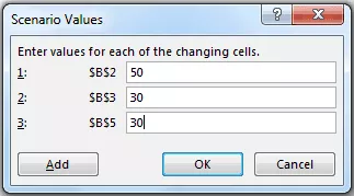
●      Select OK (Click on Add if you want to add another scenario).

For this data collection, this provides the Worst Case scenario. You can construct several situations by following these instructions in the same way (for example, Worst Case, Realistic, Best Case).

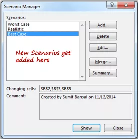
After you've finished creating all of the scenarios, double-click on any of them to see the results. The values would alter based on the scenario as you double clicked.

References:

1. Misty E. Vermaat, Microsoft word 2013 1st Edition (2013).
2. Satish Jain, M.Geeta, MS- Office 2010 Training Guide, BPB publication (2010)
3. Https://edu.gcfglobal.org/en/excel2003/moving-copying-and-deleting-cell-contents/1/
4. Https://edu.gcfglobal.org/en/excel2013/simple-formulas/1/
5. Https://www.tutorviacomputer.com/excel/use-the-function-wizard/
6. Https://www.excel-easy.com/examples/goal-seek.html