UNIT 1
Definition and Scope of Micro Economics
Microeconomics (from Greek prefix mikro- meaning "small") is a branch of economics that studies the behavior of individuals and firms in making decisions regarding the allocation of scarce resources. “The interactions among these individuals and firms”
Microeconomics is the study of individuals, households and firm’s behavior in decision making and allocation of resources. It generally applies to markets of goods and services and deals with individual and economic issues.
Definition
Microeconomics is the study of individuals, households and firms' behavior in decision making and allocation of resources. It generally applies to markets of goods and services and deals with individual and economic issues.
Microeconomics is a branch of economics that studies the behavior of individuals and firms in making decisions regarding the allocation of scarce resources and the interactions among these individuals and firms.
This is considered to be basic economics. Microeconomics may be defined as that branch of economic analysis which studies the economic behavior of the individual unit, maybe a person, a particular household, or a particular firm.
The production of goods and services is based on allocation of scarce resources.
Efficient distribution of goods – this studies the matter relating to (a) Product pricing, (b) Factor pricing, (c) Economic welfare.
- Product pricing – it involves the determination of product price under monopoly, perfect competition, etc. considering demand, supply, cost production etc.
- Factor pricing - it involves the determination of price of factor inputs such as: land, labour, capital & organization in the form of rent, wage, interest & profit respectively.
- Economic welfare – it involves the study of maximum profit for producer and maximum benefit to consumer.
Cardinal and ordinal utility analysis
Cardinal and ordinal approaches to consumer behavior determine the utility of a commodity or services. It varies according to every individual. In other words it implies the satisfying power of the goods and services. This utility is measured and can be expressed quantitatively ie 1, 3,4, 5.
Cardinal utility
Cardinal utility refers to the proposition that economic prosperity can be rightly perceived and provided with value. Individuals can determine the use of certain products consumed. It prompts measuring of the satisfactory levels in utils.
Ordinal utility
The functions that represent utility of a product according to its preference, but does not provide any numerical figure refers to ordinal utility. Ordinal utility believes that the satisfaction level cannot be evaluated; however, it can be levelled.
Difference between cardinal and ordinal utility
| Cardinal utility | Ordinal utility |
Definition | It explains that the satisfaction level after consuming a good or service can be scaled in terms of countable numbers. | It explains that the satisfaction after consuming a good or service cannot be scaled in numbers, however, these things can be arranged in the order of preference. |
Measurement | Utility is measured on the basis of utils | Utility is ranked on the basis of satisfaction |
Realistic | It is less practical. | It is more practical and sensible. |
Used by | This theory was applied by Prof. Marshall | This theory was applied by Prof. J R Hicks |
Approach | Quantitative approach | Qualitative approach |
Examination | Marginal utility analysis | Indifference curve analysis |
|
|
|
Ordinal utility indifference curve analysis
Utility analysis suffers from a flaw in the subjective nature of utility, that is, the inability to measure utility quantitatively and accurately. To overcome this difficulty, economists developed a different approach based on the indifference curve. According to this indifference curve analysis, utility cannot be accurately measured, but the consumer can state which of the combinations of two goods he prefers, without describing the magnitude of the strength of his preference. This means that if the consumer is presented with a number of different combinations of goods, he can order or rank them on a “scale of preference “if the different combinations are marked a, B, C, D, E, etc. In this case, the consumer can tell whether he likes A to B or B to A or is indifferent between them. Similarly, he can show his preference or indifference between other pairs or combinations. The concept of order utility means that consumers cannot go beyond stating their preferences or indifference. In other words, if consumers prefer A to B, they don't know by “how much “they prefer A to B. Consumers cannot state the “quantitative difference “between different satisfaction levels. He can simply compare them “qualitatively". That is, it is possible to determine whether simply one satisfaction is higher than another, or lower, or equal.
The basic tool of the Hicks-Allen order analysis of demand is the indifference curve, which represents all those combinations of goods that give the consumer the same satisfaction. In other words, all the combinations of goods that lie on the consumer's indifference curve are equally preferred by him. The independence curve is also known as the Iso-utility curve. Indifferent schedules are tabular statements showing different combinations of two goods that bring the same level of satisfaction.
Table 2.4 Indifference schedule
Combination Rice (X) Wheat (Y)

I | 1 | 12 |
II | 2 | 8 |
III | 3 | 5 |
IV | 4 | 3 |
V | 5 | 2 |
Now consumers are asked to tell the amount of wheat (Y) they are willing to give up the benefit of an additional unit of rice (X) so that the level of satisfaction remains the same. If the profit of one unit of rice fully compensates for the loss of 4 units of wheat, then the following combination of 2 units of rice
And eight units of wheat will give him as much
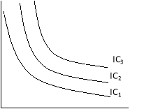
Satisfaction as the first or first combination. A set of indifferent curves representing the size of preference at different levels of satisfaction are understood because the indifferent curve map (figure 2.3).
Although the combination lying on the indifferent curve 3 (IC3) provides the same satisfaction
Product X
Commodity X
|
Fig 2.3 Indifference Curve Map
Figure 2.3 indifference curve map
The level of satisfaction in the indifference curve 3 (IC3) is greater than the level of
Satisfaction with indifference curve 2(IC2).
I) the nature of the indifference curve
A) Downward inclination: the indifference curve tilts downwards from left to right.
This means that when the amount of one good in a combination increases, the amount of another must necessarily be reduced so that the total satisfaction is constant.
If the indifference curve is a horizontal straight line (parallel to the X-axis),
Then the indifference curve is a horizontal straight line (parallel to the X-axis),
As shown in the figure. 2.4 (a) means that as the amount of good X increases,
The amount of good Y will remain constant, but the consumer will remain
Indifferent among the various combinations.
This cannot be done, because consumers always prefer
A large amount of good to a small amount of its good.
Similarly, the indifference curve cannot be a vertical straight line
Fig.2.4 (a) Horizontal Fig.2.4 (b) Vertical Fig.2.4(c) Upward Sloping Indifference Curve Indifference Curve Indifference Curve
|
A vertical straight line means that while the amount of good y in combination increases the amount of good X remains constant. The third possibility for the curve is to lean upward to the right.
Key takeaways –
- Cardinal and ordinal approaches to consumer behavior determine the utility of a commodity or services
- The functions that represent utility of a product according to its preference, but does not provide any numerical figure refers to ordinal utility.
- Microeconomics is the study of individuals, households and firm’s behavior in decision making and allocation of resources.
The law of demand states that all other factors remain constant or equal, an increase in the price causes a decrease in the quantity demanded and a decrease in goods or services price leads to increase in the quantity demanded. Thus it expresses an inverse relationship between price and demand.
For example, at Rs 70 per kg consumer may demand 2 kg of apple. On the other hand, the price rises to 100/- per kg then he may demand 1 kg of apple
Assumption of law of demand
- No change in the income
- No change in size population
- No change in price of related goods
- No change in consumers taste, preferences, etc
- No expectation of a price change in future
- No change in climate conditions
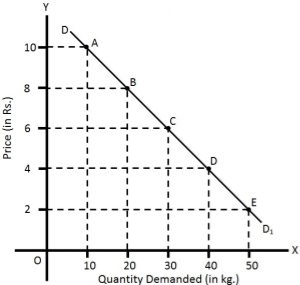
Given these assumption, the law of demand is explained in the below table –
Price(rs) | Quantity demanded |
10 | 10 |
8 | 20 |
6 | 30 |
4 | 40 |
2 | 50 |
|
The above table shows that when the price of apple, is Rs. 10 per kg, 10 kg are demanded. If the price falls to Rs.8, the demand increases to 20 kg. Similarly, when the price declines to Rs 2, the demand increases to 50 kg. This indicates the inverse relation between price and demand.
Also, in the above figure the demand curve slopes downwards as the price decreases, the quantity demanded increases.
Exception of law of demand
Under the following circumstances, consumers buy more when the price of a commodity rises, and less when price falls which leads to upward sloping demand curve.
- Giffen goods are those products where the demand increases with the increase in price. For example, necessities products like rice, wheat. Lower incomes group will spend less on superior foods (like meat) to buy more rice, wheat etc.
- In anticipation of war, consumers start buying even when the prices are high due to the fear of shortage.
- During a depression, the prices of products are low still the demand for those products is also less.
- the law of demand is not applicable on necessities of life such as food, cloth etc.
Key takeaways
- The law of demand is a fundamental principle of economics which states that at a higher price consumers will demand a lower quantity of a good.
- Demand is derived from the law of diminishing marginal utility, the fact that consumers use economic goods to satisfy their most urgent needs first.
- A market demand curve expresses the sum of quantity demanded at each price across all consumers in the market.
Under law of demand, price falls and demand rises, vice versa. But how much the quantity rise or fall for a given change in price is not determined in law of demand. So the concept of elasticity of demand is derived to know how much quantity demanded changes for a change in the price of goods or services.
“The elasticity (or responsiveness) of demand in a market is great or small according as the amount demanded increases much or little for a given fall in price, and diminishes much or little for a given rise in price”. – Dr. Marshall.
Elasticity means sensitivity of demand to the change in price.
The formula for calculating elasticity of demand is:
EP = proportional changes in quantity demanded/proportional changes in price
Types of elasticity of demand
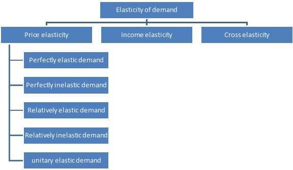
Elasticity of demand is of following types
|
Price of elasticity of demand –
- The price of elasticity demand is the change in the quantity demanded to the change in the price of the commodity
- Formula –
- Ep = percentage change in quantity demanded/percentage change in price
There are 5 types of price elasticity of demand given below
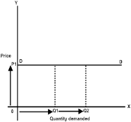
- Perfectly elastic demand
- A small change in price results to major change in demand is said to be perfectly elastic demand
- The demand curve in perfectly elastic demand represent horizontal straight line
- Ep = infinity
|
- From the above figure, we can see at price P1 consumers are ready to buy as much quantity as they want. A slight increase in price may result to fall in demand to zero.
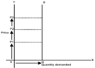
2. Perfectly inelastic demand
- When there is no change in the demand of the commodity with the change in price is said to be perfectly inelastic demand
- The demand curve in perfectly elastic demand represent Vertical straight line
- Ep = zero
|
From the above fig, we can see that price is rising from P1 to P2 to P3, but there is no change in the demand. This cannot happen in practical situation. But, in essential goods such as salt, with the change in price the demand does not change.
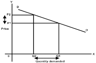
3. Relatively elastic demand
- When the proportionate change in demand is greater than the proportionate change in price of a product
- The value ranges between one to infinity (ep>1)
- Ex – a smaller change in flight price result in more demand for booking the flight tickets
|

- From the above figure, it is observed that the percentage change in demand from Q2 to Q1 is larger than the percentage change in price from P2 to P1. Thus the demand curve is gradually sloping downwards
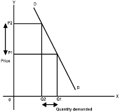
4. Relatively inelastic demand
- When the percentage change in demand is less than the percentage change in price
- The value ranges between zero to one (ep<1)
- Ex – cloths, drinks, food, oil , as the change in price does not affect the quantity demanded.
|
- From the above figure, it is interpreted that the proportionate change in demand from Q2 to Q1 is less than the proportionate change in price from P2 to P1. Thus the demand cure rapidly sloping down.
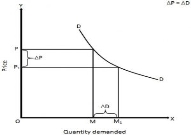
5. Unitary elastic demand
- When the percentage change in quantity demanded in equal to the percentage change in price of the commodity
- The value is equal to one (ep=1)
|
In the above figure we can observe that proportionate change in price from P to P1 cause the same proportionate change in price from M to M1
Income elasticity demand
The income elasticity is measures the sensitivity of quantity demanded for a goods or services to a change in consumer’s income
Percentage change in the consumer’s income
|
Cross elasticity
“The cross elasticity of demand is the proportional change in the quantity of X good demanded resulting from a given relative change in the price of a related good Y” Ferguson
It measures the percentage change in the quantity demanded of commodity X to the percentage change in the price of its substitute/complement Y
Proportionate change in the price of Y |
Key takeaways
- Elastic demand is when a product or service's demanded quantity changes by a greater percentage than changes in price.
- The opposite of elastic demand is inelastic demand, which is when consumers buy largely the same quantity regardless of price.
Consumers are in equilibrium when they get maximum satisfaction from the goods and are not in a position to rearrange their purchases. There is a defined apathy map showing the scale of consumer preferences across different combinations of two goods X and Y.
Consumers have a fixed income and want to spend it entirely on goods X and Y.
The price of goods X and Y is fixed to the consumer.
The goods are homogeneous and divisible.
The consumer acts rationally and maximizes his satisfaction.
Consumer equilibrium
Take his indifference curve and budget line together to show the combination of two goods X and Y that consumers buy to be balanced.
We know,
Indifferent map-shows the scale of consumer preferences between various combinations of two goods
Budget line-he shows his money income and various combinations that can afford to buy at the price of both goods.
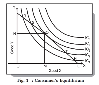
The following figure shows the indifference map with 5 indiscriminate curves (ic1, IC2, IC3, IC4, and IC5) and the budget lines PL for good X and good Y. In order to maximize his level of satisfaction, the consumer tries to reach the highest indifference curve. We assume budget constraints, so he will be forced to stay on the budget line.
|
So, what kind of combination is it?
Let's say he chose the combination R from the figure. 1, we see that R is on the low indifference curve–IC1. He can easily afford the combination S, Q, or T that is on a high Ic. Even if he chooses the combination H, the argument is similar because H is on the curve IC1.
Next, let's check out the mixture S lying on the curve IC2. Again, he can reach a better level of satisfaction within the budget by choosing the mixture Q lying on IC3–the argument is analogous for the mixture T, since the higher T is also on the curve IC2.
Therefore, we have left the combination Q.
What happens when he chooses the combination Q?
This is the simplest choice because Q is on his budget line and pts puts him on the simplest possible indifference curve, IC3. There are higher curves, IC4 and IC5, but they are over his budget. Thus, he reaches equilibrium at the point Q on the curve IC3.
Note that at this point the budget line PL is bordered by the indifference curve IC3. Also in this position, consumers buy X in OM amount and Y in ON amount.
Since Point Q is tangent, the slope of line PL and curve IC3 is equal at this point. In addition, the slope of the indifference curve shows that the substitution limit rate (MRSxy) of X with respect to Y is
Hence, at the equilibrium point Q,
MRSxy = MUxMUyMUxMUy = PxPy
Also, the slope of the price line (PL) shows the ratio of X and Y prices. Therefore, we can say that the consumer equilibrium is achieved when the price line is bordered by the indifference curve. Alternatively, when the substitution limit rate of goods X and Y is equal to the ratio between the prices of two goods.
Key takeaways - Consumers are in equilibrium when they get maximum satisfaction from the goods and are not in a position to rearrange their purchases
Price consumption curve
The price consumption curve(PCC) shows the varying amounts of products purchased by consumers as their prices change. The marshalian demand curve also shows different amounts of products demanded by consumers at various prices, while others remain an equivalent .
Given the income of the consumer's money and his indifference map, it's possible to draw a requirement curve for any commodity from the PCC.The conventional demand curve is straightforward to draw from a given price demand schedule for a commodity, whereas the drawing of the demand curve from the PCC is somewhat complicated. However, the latter method has more edges than the previous . It reaches an equivalent result without making dubious assumptions of the measurable utility of utility and therefore the constant utility of cash .
The derivation of the demand curve from the PCC also explains the income and alternative effects of a given decline or rise within the price of products that the Marshallian demand curve can't be explained. Therefore, the ordinal method for deriving the demand curve is superior to the marshalian method.
Assumption:
In this analysis、:
(a) the cash spent by the buyer is given and constant; it's Rs10.
b) the worth of an honest X falls.
(c) the costs of other related products won't change.
(d) consumer preferences and preferences are constant.
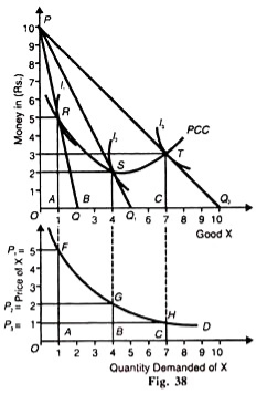
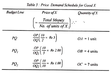
In double story figure 38, money is taken in rupees on the vertical axis and an honest X on the horizontal axis. PQ,PQ1 and PQ2 are the budget lines of consumers where R, S and T are the equilibrium positions forming the PCC curve, and if the entire gold income of consumers in OA, OB and OC units of X respectively at these points on the PCC curve divided by the amount of products purchased with it, we get per unit price of excellent . For X, OA unit, he pays OP/OQ price;for OB unit,OP/OQ1 price; and for OC unit, OP / OQ2.This is, in fact, the buyer price demand schedule for the great X shown in Table 5..
|
Consumer price demand for an honest X schedule shows that given his money income OP (Rs.10) when he spends his income on buying an oq amount (2 units), it means the worth of X is OP/OQ (Rs).5) consumers buy an honest X OA (one unit) per budget line PQ this is often indicated by the purpose R on the F curve.
if OP/OQ is valued by A, by the budget line PQ (Rs. 2), the worth consumption curve shows that he buys X OB (4 units). When the worth of excellent X is decided as OP/OQ2(=Re1)as the budget line PQ2 and therefore the curve L at the purpose T, the buyer buys OC(7 units)of X.Points R, S,and T on the PCC curve indicate the price-quantity relationship permanently X.
|
These points are plotted in the figure below figure 38. The price of X is the amount taken on the vertical axis and required on the horizontal axis. To draw a demand curve from PCC, draw a vertical from the top point R in Figure 38 to the bottom figure that should pass through point A, and then draw a line at point P1 (=5) on the price axis (figure below).
Points G and H are drawn in a similar way. This curve shows the amount of X that consumers demand at different prices. As the price of X falls, consumers buy more units of it, and the demand curve D tilts downward to the right.
Key takeaways - The price consumption curve(PCC) shows the varying amounts of products purchased by consumers as their prices change
Income consumption curve and Engel curve
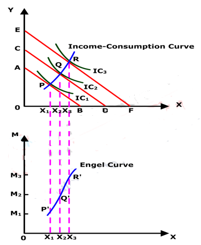
With given money income and prices of two commodities the consumer will be in equilibrium at the tangency point between the budget line and the highest indifference curve. Now, we will analyze how the situation changes and the consumer attains a new equilibrium, when income changes without any change in goods’ prices. The income consumption curve is the locus of all consumer equilibrium points resulting due to changes in consumer’s income only, with prices remaining unchanged.
In the below figure , AB indicates the budget line for a given income level (M1) and given prices. The consumer is in the equilibrium at point P when indifference curve IC1 is tangent to the budget line AB. At P, the consumer purchases OX1 of commodity X and OY1 of commodity Y. Now, suppose the income of the consumer increases from M1 to M2. With this increase in income the consumer would now be able to purchase larger quantities of both the commodities. As a result, the budget line shifts rightward, parallel to the original budget line AB. The new budget line representing M2 income level is shown by CD.
With the budget line CD the consumer reaches a new equilibrium Q on the highest possible indifference curve IC2. At Q the consumer purchases OX2 of commodity X and OY2 of commodity Y. Thus, as a result of increase in income the consumer purchases more of both the commodities. At the higher indifference curve IC2 the consumer satisfaction increases, so that he is better off at Q as compared to P. If his income increases further to M3 so that the budget line shifts to EF, the consumer reaches the indifference curve IC3 at point R and purchases greater quantities of both the commodities. If the successive consumer equilibrium points (like P, Q and R) corresponding to various level of income are connected together, we obtain the Income Consumption Curve (ICC). The Income Consumption Curve is thus the locus of the consumer’s equilibrium points corresponding to different levels of consumer’s income.
|
Engel curve
The income consumption curve can be used to derive the relationship between a consumer’s income and the quantity of goods purchased. The Engel curve shows the relationship between the consumer’s level of income and quantity purchased of a commodity, other factors remaining constant.
To derive the Engel curve from income consumption curve let us measure income levels on the vertical axis and quantity of a good purchased on the horizontal axis as in the lower panel of above Figure. The Income Consumption Curve in the top panel of above figure shows the equilibrium quantity of X and Y purchased as the income level changes. The parallel budget lines AB, CD and EF corresponds to M1, M2 and M3 level of income respectively, prices remaining constant. Each point of the ICC corresponds to a particular level of income and to a particular quantity of X (and Y). The various combinations of the income level and the quantity purchased of good X i.e. (M1, OX1), (M2, OX2) and (M3, OX3) are plotted in the lower panel to obtain the Engel curve for good X. The income-quantity combinations (M1, OX1), (M2, OX2) and (M3, OX3) shown by point P’, Q’ and R’ in the lower panel of Figure 1 correspond to the consumer’s equilibrium points P, Q and R respectively in the top panel of above figure.
In case of a normal good the consumer purchases more of it when his income increases. But an inferior good is a type of good which the consumer purchases less of when his income increases.
Above fig shows the income consumption curve and Engel curve when X is a normal good. We get a positively sloped Engel curve and income consumption curve for a normal good because the consumer purchases more of X when his income increases.
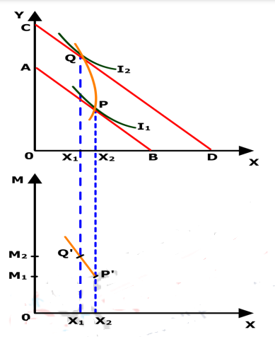
Now, let us assume X is an inferior good given in below figure. In this case, consumption of the commodity decreases as income increases. So the ICC is backward bending and the Engel curve is negatively sloped, indicating a fall in quantity purchased with an increase in income.
The income consumption curve is obtained by joining the different consumer equilibrium points as income increases from M1 to M2. As money income increases the consumer equilibrium moves from the point P on I 1to point Q on a higher indifference curve I2. At the new equilibrium Q the consumer purchases less of commodity X, which is an inferior good and more of commodity Y which is a normal good. This generates a negatively sloped income consumption curve PQ. The corresponding Engel curve is derived in the lower panel of below figure. We obtain a negatively sloped Engel curve since an increase in income leads to a decline in quantity purchased of the inferior good X.
|
Key takeaways –
- Income-consumption curve is a graph of combinations of two goods that maximize a consumer’s satisfaction at different income levels.
- The Engel curve shows the relationship between the consumer’s level of income and quantity purchased of a commodity, other factors remaining constant.
Income and substitution effect
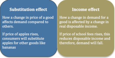
A good increase in prices will then have two different effects–known as profit and alternative effects.
If a good increase in price
- Goods are relatively more expensive than alternatives, and therefore people will switch to other goods that are relatively inexpensive. (Substitution effect)
- Higher prices reduce disposable income, and this low income can reduce demand. (Income effect)
|
Substitution effect
It states that the increase in the price of good will encourage consumers to buy alternative goods. The alternative effect measures the amount at which higher prices encourage consumers to buy different goods, assuming the same level of income.
Income effect
Thus price changes affect the interests of consumers. If prices rise, it will effectively cut disposable income and lower demand for good for disposable income this fall.
For example:
When the price of meat rises, the higher the price, consumers can switch to alternative food sources, such as buying vegetables.
But the higher the price of meat, it means that after buying some meat, they have a lower reserve income. Therefore, consumers buy less meat, but this profit.
If it goes well, it will increase like a diamond an alternative diamond for no substitution effect however, the higher the price of a diamond, the lower the demand due to the income effect.
Income and alternative effects on wages
|
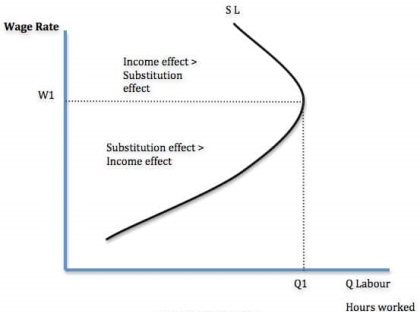
For workers, there is a choice between work and leisure.
When wages rise, work becomes relatively more profitable than leisure time. (Substitution effect)
But with higher wages, he can maintain a decent standard of living through fewer jobs. (Income effect)
The alternative effect of higher pay means workers give up their leisure time to do more hours of work because jobs now have higher rewards.
The income effect of higher wages means that workers spend less time working because they can maintain their target income level in less time.
If the alternative effect is greater than the income effect, people do more work (W1, up to Q1). But we may be at a certain hourly rate where we can afford to work less time. In the figure above, after w1, the income effect is dominant.
It depends on the workers in question. You can enjoy leisure and high-paying jobs. The income effect will soon dominate. If you have a lot of debt and spending commitments, the income effect will take a long time to occur.
Income and alternative effects for interest rates and savings
Higher interest rates increase income from savings. Thus, this will give consumers more income, which can lead to higher spending (income effect)
Higher interest rates make savings more attractive than consumption and reduce consumer spending (alternative effects)
Key takeaways –
- The income effect is the change in the consumption of goods by consumers based on their income.
- The substitution effect happens when consumers replace cheaper items with more expensive ones when their financial conditions change
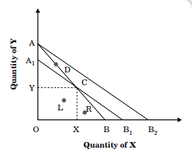
Revealed preference, a theory offered by American economist Paul Anthony Samuelson in 1938 in his article ‘Consumption Theory in Terms of Revealed Preference’, states that consumer preferences can be revealed by the purchases they make under different income and price circumstances. The revealed preference theory gives a more realistic assessment of consumer’s behavior. This theory does not take into account utility approaches or indifference curve to explain consumer behaviour. According to the revealed preference theory, the demand for a commodity by a consumer can be determined by observing the actual behaviour of the consumer with the varied levels of income and market price of commodities. The basic hypothesis of the revealed preference theory is that ‘choice reveals preference’. The theory explains the demand curve on the basis of consumer’s behavior.
Assumption
- The consumer has only two combinations of commodities
- The income of the consumer, prices of the two commodities are constant during the period of analysis
- The tastes of the consumer are given and remain unchanged during the period of analysis
- The consumer should choose only one combination of the commodities in a given price-income situation
- Based on observed facts and ordinal utility analysis
- A consumer can be persuaded to buy more of a commodity if its price is subjected to substantial cut
- The choice of the consumer reveals his preference and market behaviour of the consumer
- Consistency states strong ordering preference hypothesis of Samuelson
- Transitivity states that no two observations of choice behaviour can conflict with regard to an individual consumer’s preferences.
|
From the above figure, AB is the budget line. Therefore, OAB is the feasible set where all points on or below AB can be attained by the consumer with the given income and market price of commodities. Suppose the consumer chooses C of all the possible combinations of commodities X and Y. This implies that the consumer has revealed his/her preference for combination C over all other combinations, which are D, L, and R.
There are three main axioms proposed under the revealed preference theory as follows
- Weak Axiom of Revealed Preference (WARP): As per this axiom, a consumer always makes the same choice while purchasing one commodity instead of the other at the given price and income. The consumer makes a different choice if the other commodity provides more benefit in terms of more affordability or better quality.
- Strong Axiom of Revealed Preference (SARP): The SARP applies the concept of transitivity to revealed preferences. This implies that if a consumer chooses commodity A over commodity B and commodity B over commodity C, the consumer would prefer commodity A to commodity C. ‰
- Generalised Axiom of Revealed Preference (GARP): This axiom states that more than one combination of two commodities provides the same level of satisfaction to a consumer at a given market price and income level. As per GARP, there is no unique combination of two commodities that provides maximum utility to the consumer.
Key takeaways –
- Revealed preference is an economic theory regarding an individual's consumption patterns, which asserts that the best way to measure consumer preferences is to observe their purchasing behavior.
Sources
1. Lipsey, R.G. and K.A. Chrystal, Economics, Oxford Printing Press
2. Bilas, Richard A. Microeconomic Theory: A Graphical Analysis, McGraw Hill book Co.
Kogakusha co. Ltd.
3. Amit Sachdeva, Micro Economics, Kusum Lata Publishers.
4. Chopra, P.N. Micro Economics
5. Seth, M.L. Micro Economics
