UNIT 2
Production function
Production function
To have clear knowledge about production and cost it’s mandatory to know the basics of production functions and understand the fundamentals in mathematical terms. We break down short-term and long-term production functions supported variable and glued factors.
What is the production function?
The functional relationship between the physical input (or factor of production) and therefore the output is named a production function. It assumed the input as an explanatory or independent variable and the output as a dependent variable. Mathematically, you can write this as:
Q=f(L,K)
Where"Q"represents the output,"L"and"K" are the inputs, respectively, labour and capital (such as machinery). Note that there may be many other factors, but we are assuming a two-factor input here. Production functions are defined differently in the short term and in the long term. This distinction is crucial in microeconomics. This distinction is based on the nature of the factor input.
Inputs that change directly with the output are called variable factors. These are factors that can change. Fluctuating factors exist both in the short term and in the long term. Examples of variable factors include daily labour and raw materials.
On the other hand, factors that cannot change or change as the output changes are called fixed factors. These factors are usually characteristic only for a short or short period of time. There are no fixed factors in the long term.
Therefore, two production functions can be defined: short-term and long-term. A short-term production function defines the connection between one variable factor (keeping all other factors fixed) and therefore the output. The law of regression to factors explains such a production function.
For example, suppose that a company has 20 units of Labour and 6 acres of land, and initially uses only Labour units (variable coefficients) for that land (fixed coefficients). Thus, the ratio of land and labour is 6: 1. Now, if the company chooses to adopt 2 labour units, then the ratio of land to Labour will be 3: 1 (6: 2).
Here, all factors change in the same proportion. The law used to explain this is called the law of return to scale. It measures how much of the output changes when the input changes proportionally.
|
Key takeaways –
- The functional relationship between the physical input (or factor of production) and therefore the output is named a production function
Law of variable proportion
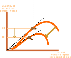
The law of variable proportion states that keeping all other factors fixed, when the quantity of one factor increased, the marginal product of that factor will eventually decline. This means that upto the use of a certain amount of variable factor, marginal product of the factor may increase and after a certain stage it starts diminishing. When the variable factor becomes relatively abundant, the marginal product may become negative.
Definition
“As the proportion of the factor in a combination of factors is increased after a point, first the marginal and then the average product of that factor will diminish.” Benham
Assumption
The following assumption of law of variable proportion
- The state of technology is assumed to be constant
- Fixed amount of other factors
- The law is based upon the possibility of varying the proportions in which the various factors can be combined to produce a product.
Illustration of the Law:
The law of variable proportion is explained in the below given table and figure. Assume that a there is a given fixed amount of land, in which more labour (variable factor) is used to produce agricultural product.
Units of labour | Total product | Marginal product | Average product |
|
1 | 2 | 2 | 2 |
|
2 | 6 | 4 | 3 |
|
3 | 12 | 6 | 4 |
|
4 | 16 | 4 | 4 |
|
5 | 18 | 2 | 3.6 |
|
6 | 18 | 0 | 3 |
|
7 | 14 | -4 | 2 |
|
8 | 8 | -6 | 1 |
|
In the above table we can observe that upto the use of 3 units of labour, total product increases at an increasing rate. But after the third unit total product increases at a diminishing rate.
A marginal product is the incremental change in total product as a result of increasing the variable factor i.e labour. We can see from the table, marginal product of labour initially rises and beyond the use of third unit it starts diminishing. The use of 6 units does not add anything in the production. Thus marginal product of labour fallen to zero. After the 6 unit, total product decreases and marginal product becomes negative.
Average product is derived by dividing total product by the quantity of variable unit. Till the 3 unit of labour, average product increases. Whereas after the 3 unit, average product is falling throughout.
Three Stages of the Law of Variable Proportions:
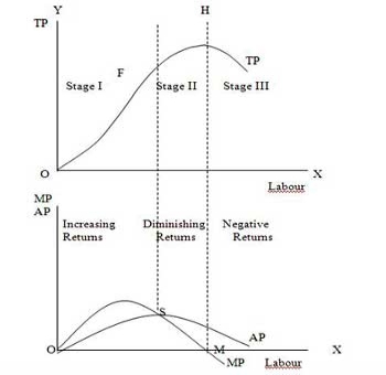
The stages are discussed in the below figure where labour is measured on the X-axis and output on the Y-axis.
|
Stage 1. Stage of Increasing Returns:
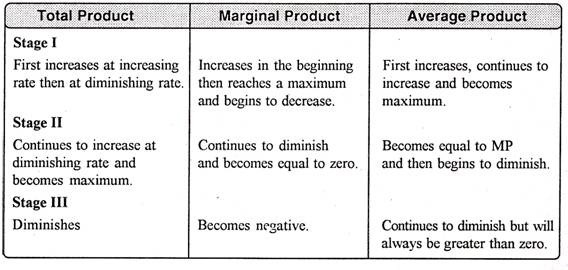
In this stage, total product increases at an increasing rate till point F..ie the curve TP concave upwards upto point F which means marginal product of labour rises. Because efficiency of fixed factor increases with the increase in variable facto labour. After point F, the total product starts increasing at a diminishing rate. Looking at the next figure, marginal product of labour is maximum, after which it diminishes. This stage is called the stage of increasing returns because the average product of the variable factor labour increases throughout this stage. This stage ends at the point where the average product curve reaches its highest point.
Stage 2. Stage of Diminishing Returns:
The stage 2 ends, when the total product increases at a diminishing rate until it reaches it maximum point H. In this stage both marginal product and average product are diminishing but remain positive. Because fixed factor land becomes inadequate with the increase in the quantity of variable factor labour. At point M marginal product is zero which corresponds to the maximum point H of the total product curve.
Stage 3. Stage of Negative Returns:
In stage 3, with the increase in variable factor labour, the total product decline. Therefore the TP curve slopes downward. As a result, marginal product of labour is negative and MP cure falls below x axis. In this case fixed factor land becomes too much inadequate to the increase in variable factor labour.
|
Key takeaways –
- The law of variable proportion states that keeping all other factors fixed, when the quantity of one factor increased, the marginal product of that factor will eventually decline.
- Three stages are increasing return, diminishing return and negative return
Return of scale
In long run, no factors are fixed. Return of scale refers to proportionate change in productivity from proportionate change in all the inputs.
Definition:
“The term returns to scale refers to the changes in output as all factors change by the same proportion.” Koutsoyiannis
“Returns to scale relates to the behaviour of total output as all inputs are varied and is a long run concept”. Leibhafsky
Types of return of scale
1. Increasing return of scale
2. Constant return of scale
3. Diminishing return of scale
Explanation
- Increasing return of scale
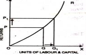
- When proportionate increase in factors of production leads to higher proportionate increase in production refers to increasing return of scale.
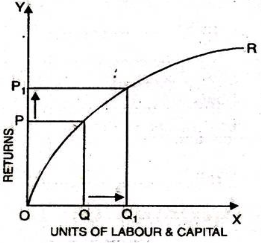
- In the below figure, x axis represent increase in labour and capital while Y axis represent increase in output. When labour and capital increases from Q to Q1, output also increases from P to P1 which is higher than the change in factors of production ie labour and capital
|
2. Diminishing return of scale
- Diminishing return refers to percentage increase in factors of proportion leads to smaller proportion increase in the output
- For instance, 30% increase in variable input (labour and capital) result in 10% increase in output.
- In the below diagram, x axis refers increase in labour and capital while Y axis refers increase in output. Percentage increase in labour and capital from Q to Q1 results in less percentage change in output from P to P1
|
3. Constant return of scale
- Constant return of scale refers to output increases in same proportion in which factors of production (labour and capital) increases.
- Internal and external economies is equal to internal and external diseconomies
- This is known as homogenous production function
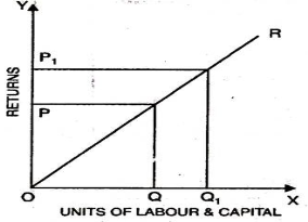
- In the below figure, x axis refers increase in labour and capital while Y axis refers increase in output. Increase in labour and capital from Q to Q1 is equal to the increases in output from P To P1
|
Key takeaways –
- Return of scale refers to proportionate change in productivity from proportionate change in all the inputs
Isoquants
These lines represent various input combinations which produce the same levels of output. The producer can choose any of these combinations available to him because their outputs are always the same. Thus, we can also call them equal product curves or production indifference curves.
Just like indifference curves, isoquants are also negatively-sloping and convex in shape. They never intersect with each other. When there are more curves than one, the curve on the right represents greater output and curves on the left show less output.
Consider the table below. It shows four combinations, i.e. A, B, C and D, which produce varying levels of output.
Factor combinations Units of Labour Units of Capital
A 5 9
B 10 6
C 15 4
D 20 3
Plotting these figures on a graph provides us with this curve (Figure 1):
The X-axis shows units of labour, while the Y-axis represents units of capital. Points A, B, C and D are combinations of factors on which IQ is the level of output, i.e. 100 units. IQ1 and IQ2 represent greater potential output.
Isocost Lines
Isocost lines represent combinations of two factors that can be bought with different outlays. In other words, it shows how we can spend money on two different factors to produce maximum output. These lines are also called budget lines or budget constraint lines.
Let’s assume that a farmer has Rs. 1,000 to spend on labour costs and ploughs for farming. The cost of one such plough and wage per labourer is Rs. 100. Considering his total outlay of Rs. 1,000, he can spend that money in the following combinations:
Ploughs | 0 | 100 | 200 | 300 | 400 | 500 | 600 | 700 | 800 | 900 | 1000 |
Labour | 1000 | 900 | 800 | 700 | 600 | 500 | 400 | 300 | 200 | 100 | 0 |
The farmer, in this case, can either spend the entire sum of Rs. 1,000 on just ploughs by buying 10 of them. Similarly, he can also spend it all on labour by employing 10 labourers. He can even purchase both, labour and ploughs using different combinations as shown above. The total outlay of Rs. 1,000 will remain the same. Hence, the isocost line will remain straight as shown below:
|
The x-axis represents units of ploughs, and Y-axis would show units of labour. Output levels are shown by a straight line because they remain constant.
Marginal rate of technical substitution
Marginal rate of technical substitution refers to rate, at which one
input can be substituted for another input, without affecting the total output. Capital and labour are two inputs, in case amount of capital that can be replaced by an extra unit of labour, keeping the output constant.
Marginal rate of technical substitution of labour for capital = slope = ∆K/∆L
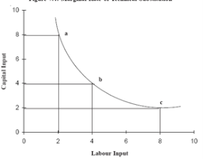
Factor combination | Unit of labour | Unit of capital | MRTS of L for K |
A | 2 | 8 |
|
B | 4 | 4 | (4-8)/(4-2) = 2 |
C | 8 | 2 | (2-4)/(4-8) = 1/2 |
|
|
|
|
|
Capital and labour are not perfect substitutes for each other so The MRTS has decreased. Therefore , while keeping the output level constant, more of labour is added, less of capital can be used.
Since, by definition, output remains constant on an isoquant the loss in physical output from a small reduction in capital will be equal to the gain in physical output from a small increment in labour.
The loss in output is calculated by multiplying the marginal physical product of capital (MP) by the amount of reduction in capital. The gain in output is calculated by multiplying the marginal physical product of labour (MP by the increment in labour.
Accordingly, along an isoquant:
∆K.MPK + ∆L.MPL = 0
∆K x MPK = ∆L x MPL
∆K/∆L = MPL/MPK
But ∆K/∆L, by definition, is the marginal rate of technical substitution of labour for capital
Therefore, MRTSLK = MPL/MPK
Thus we can see that marginal rate of technical substitution of labour for capital is the ratio of marginal physical product of the two factors labour and capital.
Economic region of production
Economic region a territorial component of a country’s national economy. Economic region is characterised by specific economic-geographical status, by an economic unity, by distinctive natural and economic conditions, and by a production specialization based on territorial social division of labor. Under capitalism, in the heat of competition economic regions form and develop spontaneously. Under socialism, based on the economic laws of socialism, the territorial division of labor develops, and economic regions form develops in a planned fashion.
In the formation of economic regions, specialization within the social territorial division of labor plays the principal role. The boundaries of a region is determined by the specialised branches action and major auxiliary facilities—the associated cooperative suppliers of raw materials, assemblies, and parts.
Economic region is also influenced by natural conditions such as the natural fertility of the soil, and the climate, the presence of large deposits of minerals.
Other factors influencing the economic region formation are administrative and political units , technical and economic conditions.
The three levels of economic regions are as follows: large (macroregions), administrative (mesoregions), and lowest-level (microregions).
Large economic regions comprise three types: Union republics, groups of Union republics, and groups of autonomous republics. The large economy determines territorial proportions of national economies. It also determines the trends in the location of productive forces throughout the national economy.
Administrative economic regions form the basis of the country’s territorial makeup. It includes the basic elements in the territorial planning and management of the national economy.
Lowest-level economic regions are low-level administrative regions that include the primary territorial elements in the classification of economic regions.
Optimum factors of production
Optimum factors of production are explained in two methods are as follows
- Marginal product approach – in the long run, a firm uses varied amount of factors in the production of goods. The factors includes what technique of production to use, what design of factory to build, what type of machinery to buy. The profit maximisation will choose the lowest cost combination of factors. When the money spent on each factors brings the equal revenue, the profit of a firm is maximised.
Formula:
Mppa = Mppb = Mppc = Mppn Pa Pb Pc Pn
|
Where as,
a, b, c, n are different factors of production.
Mpp is the marginal physical product.
A firm compares the Mpp / P ratios with that of another. A firm will reduce its cost by using more of those factors with a high Mpp / P ratios and less of those with a low Mpp / P ratio until they all become equal.
2. The isoquant approach - The least cost combination of-factors is explained with the help of iso-product curves and isocosts. The optimum factors combination or the least cost combination refers to the combination of factors to produce a specific quantity of output at the lowest possible cost. The least cost combination of factors for any level of output when the iso-product curve is tangent to an isocost curve
The choice of a particular combination of factors depends on technical possibilities of production and the prices of factors used for the production of a particular product.
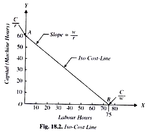
The prices of factors are represented by the iso-cost line. The Iso cost line is very important in determining what combination of factors the firm will choose for production
For ex, a firm has to spend 300/-on the factors of production such as labour and capital. Price of labour is Rs. 4 per labour hour and the price of capital is Rs. 5 per machine hour. With outlay of Rs. 300, a firm can buy 75 units of labour or 60 units capital). In the below figure, OB represent 75 units of labour and OA represent 60 units of capital.
|
This line AB is called iso-cost line, the combination of various factors which a firm can buy with a constant outlay. The iso-cost line is also called the price line or outlay line.
Assumption of optimum factor combination
- There are two factors X and Y in the combinations.
- All the units of factor X and Y are homogeneous
- The prices of factors X and Y are given and constants.
- The total money outlay is also given.
- In the factor market, it is the perfect completion which prevails.
- The isoquant must be convert to the origin.
- The slope of the Isoquant must be equal to the slope of isocost line.
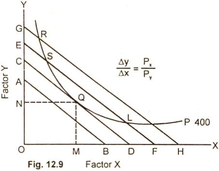
The optimum factor combination is explained in the below diagram
|
The entrepreneur decides to produce 400units of output which is represented by isoquant P. The 400 unit of output can be produced by any combination of factor X(labour) and Factor Y (capital) such as R, S, Q, L and P lying on the isoquant. For producing 400 units, the cost will be minimum at point Q, which the iso-cost line CD is tangent to the given isoquant. At no other point such as R, S,L, P the cost is minimum. Therefore the firm will not choose any combination of R,S,L,P.
Expansion path
In economics, an expansion path is a line connecting optimal input combinations as the scale of production expands. A producer seeking to produce the most units of a product in the cheapest possible way to increase production along the expansion path.
Definition
Economist Alfred Stonier and Douglas Hague defined expansion path as,” that line which reflects least cost method of producing different levels of output, when factor prices remains constant”.
Assumption
- There are two factors of production, labour and capital, which are variable.
- All units of labour and capital are homogeneous
- The price of labour is constant
- The price of capital is constant
- The firm increases its total outlay in order to expand its output.
In order to maximise profits, the firm combines labour and capital in such a way that the ratio of their MP is equal to the ratio of their prices
|
This occurs at a point of tangency between an isocost line and an isoquant curve.
|
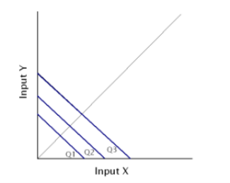
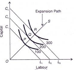
In the above figure, the different isoquant lines areC1L1,C2L2,C3L3. Keeping the prices of factors constant, the different isoquant lines are shown parallel to each other. There are three isoquants ie 100, 200, 300 representing successively higher level of output.
At point P, the firm is at equilibrium, where the isoquant 100 is tangent to its corresponding isoquant line C1L1. Similarly the firm is equilibrium at point Q and R, where the isoquant 200 and 300 is tangent to its corresponding isoquant line C2L2 and C3L3. Each point of tangency implies optimum combination of capital and labour that produces optimum level of output. The line OS joining the equilibrium point P,Q,R from the origin is the expansion path of the firm.
Key takeaways –
- An isoquant, in microeconomics, is a contour line drawn through the set of points at which the same quantity of output is produced while changing the quantities of two or more inputs.
- An expansion path is a line connecting optimal input combinations as the scale of production expands.
- Economic region is characterised by specific economic-geographical status, by an economic unity, by distinctive natural and economic conditions, and by a production specialization based on territorial social division of labor.
Social and private costs of production
Private cost are the those costs that are incurred by the individuals and firms who are directly involved in some economic activity. When goods and services are produced, then certain direct and indirect costs are borne by the producing agents. Examples of private costs are the factors payments made and expenditure on raw materials incurred by the producing agent concerned.
Social cost are the costs incurred by the society as a whole. These are the private costs plus any costs borne by the rest of the society. So social costs are higher than private costs when firms are able to escape some of the economic costs of production. Such a situation is called negative externalities. Noise pollution, water pollution etc. are examples of social costs. Private costs can be made equal to social costs by public regulation that requires the firm to install anti-pollution equipment.
Long run and short run cost of production
Cost behavior in the short term
Short-term costs are important for understanding costs in economics. Short-term and long-term distinctions based on fixed and variable factors of production make the concept of understanding short-term costs easier. Let us understand the concept using examples, diagrams for graphical representation.
Short run concept
To understand short-term costs, it is important to understand the concept of short-term costs. In economics, we distinguish between short-term and long-term through the application of fixed or variable inputs.
Fixed input (plant, machine, etc.)) is a factor of production that can not be changed or changed in a short span because the period is"too small". This will be short-term. Here, the inputs are two types: fixed and variable.
In the long run, all inputs will be mutable(e.g.. Raw materials). This means that all inputs can be changed as the output volume changes. Therefore, the concept of fixed input applies only in the short term. It is in the short-term cost that we turn this time.
It explains that the cost of production depends on the level of output, given that others remain the same (ceteris paribus). This can be mathematically written as:
C=f(X)
Where C is the production cost and X is the output level.
Total fixed costs
Fixed cost refers to the cost of fixed input. At the level of output it does not change (hence, fixed). Fixed inputs include buildings,machines, etc. Thus, the cost of inputs, such as rent and the cost of machines, constitute a fixed cost. Also known as overhead, supplemental or overhead, these costs remain the same regardless of the level of output.
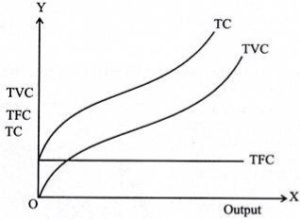
So if you plot the total fixed cost (TFC) curve against the output level on the horizontal axis, you get a straight line parallel to the horizontal axis. This indicates that these costs remain the same and should occur even if the output level is zero.
Total variable costs
The costs incurred by variable factors in production are called Total variable costs(TVC). These costs differ in the level of output. Therefore, when the production level is zero, the TVC is also zero. Thus, the TVC curve begins at the origin.
The Shape of the TVC is unique. It is said that it has the form of an inverted S. This is because, in the early stages of production, there is a scope for efficient use of fixed factors by using more variable factors (e.g., variable factors). Workers who use the machine).
Thus, as the variable input used increases, the production efficiency of the variable input ensures at a rate at which the TVC increases but decreases. This makes the first part of the tvc curve concave.
As production continues to increase, more variable factors are employed for a given amount of fixed inputs. The production efficiency of each variable factor is reduced,adding more to the production cost. Therefore, TVC will increase,but now it is increasing at the rate of increase. This is where the shape of the TVC curve is convex. Thus, the TVC curve will have an inverted-S shape.
Total cost
Total cost(TC) refers to the sum of fixed and variable costs incurred in the short term. So, the short-term cost can be expressed as follows
TC=TFC+TVC
Note that in the long run, TFC=0, so TC = TVC. So you can get the shape of the TC curve by summing the TFC curve and the TVC curve.
|
For the TC curve, the following points can be noted:
- The TC curve is shaped of reverse S. This is because of the TVC curve. Since the TFC curve is horizontal, the difference between the TC curve and the TVC curve is the same at each level of the output and is equal to the tfc. This is explained as follows: TC-TVC=TFC
- The TFC curve is parallel to the horizontal axis, and the TVC curve is inverted S-shaped.
- The law that explains the Shape of TVC and subsequent TC is called the law of variable proportions.
Economies and diseconomies of scale
Economies of scale are defined as cost advantages that an organization can achieve by expanding its production over the long term.
In other words, these are the benefits of large-scale production of the organization. Cost benefits are achieved in the form of a low average cost per unit.
It's a long-term concept. Economies of scale are achieved when the turnover of the organization increases. As a result, the savings of the organization will increase, and it will be even more possible for the organization to obtain large amounts of raw materials. This will help the organization to enjoy discounts. These benefits are called economies of scale.
Economies of scale are divided into internal and external economies, which are discussed as follows:
i.Internal economy:
See the real economy arising from the expansion of the plant size of the organization. These economies arise from the expansion of the organization itself.
An example of an economy of internal size is:
a.Technical economy of scale:
It occurs when an organization invests in expensive and advanced technologies. This helps to reduce and control the production costs of the organization. These economies are enjoyed due to the technical efficiency obtained by the organization. Advanced technology allows organizations to produce a large number of goods in a short time. Thus, the industry-wide economy falls per unit of production costs
b.Marketing economy of scale:
Scale marketing economy is achieved in case of bulk purchase, branding, and advertising when large organizations have broadened their marketing budgets over large output. For example, large organizations enjoy the benefits of advertising costs as they cover a larger audience. On the other hand, small organizations pay the same advertising costs as big ones, but do not enjoy such benefits in advertising costs.
c.Financial economy of scale:
This happens when large organizations borrow money at a lower rate of interest. These organizations have good credibility in the market. In general, banks prefer to grant loans to organizations that have a strong foothold in the market and have good repayment capacity.
d.Management economy of scale:
During the occurrence of large organizations specialized workers for different things. These workers are experts in their respective fields and use their knowledge and experience to maximize the benefits of the organization. For example, in an organization, accounts and research departments are created and managed by experienced individuals so that all costs and benefits of the organization can be properly estimated.
E.Commercial economy:
See an economy where organizations enjoy the benefits of purchasing raw materials and selling finished products at a lower cost. Large organizations buy raw materials in bulk; therefore, enjoy the advantages of transportation charge from Bank, easy credit, and prompt delivery of products to customers.
ii.Foreign economy:
Occurs outside the organization. These economies arise within industries that benefit organizations. If the industry expands, the organization will benefit from better transport networks,infrastructure and other facilities. This will help reduce the cost of the organization.
Some examples of economies of external scale are discussed as follows:
A.Economy of concentration:
See the economy resulting from skilled labor, better credit, and the availability of transport facilities.
B.Economy of information:
Means the benefits gained from trade and business related publications. The central research institution is the source of information for the organization.
C.Collapsing economy:
Refer to the division of associations caused by the economic process into different processes.
Uneconomics of scale occurs when the long-term average cost of an organization increases. It can occur when the tissue becomes excessively large. In other words, uneconomics of Scale Causes larger org-anizations to produce goods and services at increased costs.
There are two types of scale diseconomies: internal diseconomies and external diseconomies, which are discussed as follows:
i.Internal uneconomics of the scale:
See uneconomical raising the cost of production in the organization. The main factors affecting the cost of production of the organization include the lack of determination, supervision and technical difficulties.
ii.External uneconomics of the scale:
See uneconomical to limit the expansion of an organization or industry. Factors acting as restraints on expansion include increased production costs, a shortage of raw materials and a decline in the supply of skilled workers.
There are several causes of diseconomics of scale.
Some of the causes that lead to uneconomics of scale are:
i.Act as the main reason for diseconomics of scale.
If the organization's production goals and objectives are not properly communicated to employees in the organization, they can lead to overproduction or production. This can lead to diseconomics of scale.
Separately, if the communication process in the organization is not strong, then the employee will not get enough feedback. As a result, there will be less face-to-face interaction between employees, which will affect the production process.
ii.Lack of motivation:
This leads to a decrease in productivity levels. For large organizations, workers may feel isolated and less motivated because they are less valued for their work. Because of poor communication networks, it is difficult for employers to interact with employees and build a sense of attributes. This leads to a decrease in the productivity level of output due to lack of motivation. This further leads to an increase in the cost of the organization.
iii.Loss of control:
It serves as the main problem of large organizations. Monitoring and controlling the work of all employees in a large organization becomes impossible and expensive. It is difficult to make sure that all employees of the organization are working towards the same goal. It becomes difficult for managers to direct the sub-coordinates of large organizations.
iv.Cannibalism:
It means a situation where an organization is facing competition from its products. While smaller organizations face competition from the products of other organizations, larger organizations find their products compete with each other.
Economies of scope
Economies of scope is an economic concept that the unit cost to produce a product will decline as the variety of products increases. That means, the more different-but-similar goods you produce, the lower the total cost to produce each one.
For example, a shoe manufacture produces men’s and women’s sneakers. If he adds a children’s line of sneakers would increase economies of scope because to make a new line of products he can use the same production equipment, supplies, storage, and distribution channels. Thus the cost of production will be reduced.
In such case due to the production of complemetary goods and services the long run average and marginal cost of the company decreases.
Key takeaways
- Economies of scope describe situations where producing two or more goods together results in a lower marginal cost than producing them separately.
- Private cost are the those costs that are incurred by the individuals and firms who are directly involved in some economic activity.
- Social cost are the costs incurred by the society as a whole
- Economies of scale are defined as cost advantages that an organization can achieve by expanding its production over the long term
Sources
1. Lipsey, R.G. and K.A. Chrystal, Economics, Oxford Printing Press
2. Bilas, Richard A. Microeconomic Theory: A Graphical Analysis, McGraw Hill book Co.
Kogakusha co. Ltd.
3. Amit Sachdeva, Micro Economics, Kusum Lata Publishers.
4. Chopra, P.N. Micro Economics
5. Seth, M.L. Micro Economics
