Unit - 1

Introduction

1.1 Basic Terminologies, Data Structure

A data structure is a collection of data pieces that provides an efficient method for storing and organizing data in a computer so that it may be used effectively. Arrays, Linked Lists, Stacks, Queues, and other Data Structures are examples. Data Structures are employed in practically every element of computer science, including operating systems, compiler design, artificial intelligence, graphics, and many more applications.

Data Structures are an important aspect of many computer science algorithms because they allow programmers to efficiently handle data. It is critical to improving the performance of a software or program because the software's primary duty is to save and retrieve user data as quickly as feasible.

The building blocks of every program or software are data structures. The most challenging challenge for a programmer is deciding on a suitable data structure for a program. When it comes to data structures, the following terminology is utilized.

Data: The data on a student can be defined as an elementary value or a set of values, for example, the student's name and id.

Group items: Group items are data items that include subordinate data items, such as a student's name, which can have both a first and a last name.

Record: A record can be characterized as a collection of several data objects. For example, if we consider the student entity, the name, address, course, and grades can all be gathered together to constitute the student's record.

File: A file is a collection of various records of one type of entity; for example, if there are 60 employees in the class, the relevant file will contain 20 records, each containing information about each employee.

Attribute and Entity: A class of objects is represented by an entity. It has a number of characteristics. Each attribute represents an entity's specific property.

Need of Data Structures

As applications are getting complexed and amount of data is increasing day by day, there may arise the following problems:

Processor speed: To handle very large amount of data, high speed processing is required, but as the data is growing day by day to the billions of files per entity, processor may fail to deal with that much amount of data.

Data Search: Consider an inventory size of 106 items in a store, If our application needs to search for a particular item, it needs to traverse 106 items every time, results in slowing down the search process.

Multiple requests: If thousands of users are searching the data simultaneously on a web server, then there are the chances that a very large server can be failed during that process

In order to solve the above problems, data structures are used. Data is organized to form a data structure in such a way that all items are not required to be searched and required data can be searched instantly.

Advantages of Data Structures

Efficiency: Efficiency of a program depends upon the choice of data structures. For example: suppose, we have some data and we need to perform the search for a particular record. In that case, if we organize our data in an array, we will have to search sequentially element by element. Hence, using array may not be very efficient here. There are better data structures which can make the search process efficient like ordered array, binary search tree or hash tables.

Reusability: Data structures are reusable, i.e. once we have implemented a particular data structure, we can use it at any other place. Implementation of data structures can be compiled into libraries which can be used by different clients.

Abstraction: Data structure is specified by the ADT which provides a level of abstraction. The client program uses the data structure through interface only, without getting into the implementation details.

Types of data structure with its properties and operations

Types of data structure

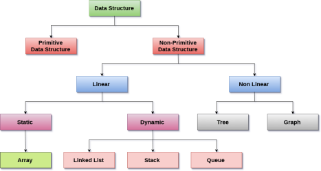
Linear data structure

In Data structure is linear. The processing of data items can be done in a linear fashion, that is, one by one. A linear structure is a data structure that can hold a large number of objects. The things can be added in a variety of ways, but once added, they maintain a constant relationship with their neighbors. For example, a collection of numbers, a collection of strings, and so on.

Once an item is added, it remains in its current location in relation to the things that came before and after it.

Example

●      Array

●      Linked list

●      Stack

●      Queue

Array

An array is a collection of data elements of similar types, each of which is referred to as an element of the array. The element's data type can be any valid data type, such as char, int, float, or double.

The array's elements all have the same variable name, but each one has a different subscript number. One-dimensional, two-dimensional, or multidimensional arrays are all possible.

The age array's individual elements are as follows:

Age[0], age[1], age[2], age[3],......... Age[98], age[99].

Linked list

A linked list is a type of linear data structure that is used to keep track of a list in memory. It's a collection of nodes that are stored in non-contiguous memory regions. Each node in the list has a pointer to the node next to it.

Stack

A stack is a linear list with only one end, termed the top, where insertions and deletions are permitted.

A stack is an abstract data type (ADT) that can be used in a variety of programming languages. It's called a stack because it behaves like a real-life stack, such as a stack of plates or a deck of cards.

Queue

A queue is a linear list in which elements can only be added at one end, called the back end, and deleted at the other end, called the front end.

It's a data structure that's similar to a stack. Because the queue is open on both ends, the data items are stored using the First-In-First-Out (FIFO) approach.

Non - linear data structure

The processing of data items in a non-linear data structure is not linear.

Example

●      Tree

●      Graph

Tree

Trees are multilevel data structures containing nodes that have a hierarchical relationship between them. Leaf nodes are at the bottom of the hierarchical tree, whereas root nodes are at the top. Each node has pointers that point to other nodes.

The parent-child relationship between the nodes is the basis of the tree data structure. Except for the leaf nodes, each node in the tree can have several children, although each node can only have one parent, with the exception of the root node.

Graph

Graphs can be defined as a graphical depiction of a collection of elements (represented by vertices) connected by edges. A graph differs from a tree in the sense that a graph can have a cycle, but a tree cannot.

Operations

1. Traversing

The set of data elements is present in every data structure. Traversing a data structure is going through each element in order to perform a certain action, such as searching or sorting.

For example, if we need to discover the average of a student's grades in six different topics, we must first traverse the entire array of grades and calculate the total amount, then divide that sum by the number of subjects, which in this case is six, to find the average.

2.     Insertion

The process of adding elements to the data structure at any position is known as insertion.

We can only introduce n-1 data elements into a data structure if its size is n.

3.     Deletion

Deletion is the process of eliminating an element from a data structure. We can remove an element from the data structure at any point in the data structure.

Underflow occurs when we try to delete an element from an empty data structure.

4.     Searching

Searching is the process of discovering an element's location within a data structure. There are two types of search algorithms: Linear Search and Binary Search.

5.     Sorting

Sorting is the process of putting the data structure in a specified order. Sorting can be done using a variety of algorithms, such as insertion sort, selection sort, bubble sort, and so on.

6.     Merging

Merging occurs when two lists, List A and List B, of size M and N, respectively, containing comparable types of elements are combined to form a third list, List C, of size (M+N).

Key takeaway

A data structure is a collection of data pieces that provides an efficient method for storing and organizing data in a computer so that it may be used effectively.

Arrays, Linked Lists, Stacks, Queues, and other Data Structures are examples.

Data Structures are an important aspect of many computer science algorithms because they allow programmers to efficiently handle data.

1.2 Analysis of an Algorithm

Analysis is the theoretical way to study performance of computer program. Analysis of an algorithm is helpful to decide the complexity of an algorithm.  There are three ways to analyze an algorithm which are stated as below.

1. Worst case: In worst case analysis of an algorithm, upper bound of an algorithm is calculated. This case considers the maximum number of operation on algorithm. For example if user want to search a word in English dictionary which is not present in the dictionary. In this case user has to check all the words in dictionary for desired word.

2. Best case: In best case analysis of an algorithm, lower bound of an algorithm is calculated. This case considers the minimum number of operation on algorithm. For example if user want to search a word in English dictionary which is found at the first attempt. In this case there is no need to check other words in dictionary.

3. Average case: In average case analysis of an algorithm, all possible inputs are consider and computing time is calculated for all inputs. Average case analysis is performed by summation of all calculated value which is divided by total number of inputs. In average case analysis user must be aware about the all types of input so average case analysis are very rarely used in practical cases.

1.3 Asymptotic Notations

To express the running time complexity of algorithm three asymptotic notations are available. Asymptotic notations are also called as asymptotic bounds. Notations are used to relate the growth of complex functions with the simple function. Asymptotic notations have a domain of natural numbers.

Big Oh (O) Notation:

• It is the formal way to express the time complexity.
• It is used to define the upper bound of an algorithm’s running time.
• It shows the worst-case time complexity or largest amount of time taken by the algorithm to perform a certain task.

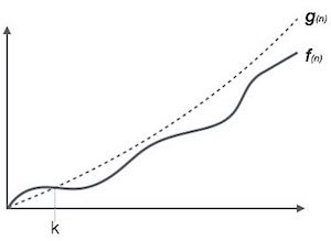
Fig: Big Oh notation

Here, f (n) <= g (n) …………….(eq1)

        where n>= k, C>0 and k>=1

If any algorithm satisfies the eq1 condition then it becomes f (n)= O (g (n))

Consider the following example

In the above example g(n) is ‘’n’ and f(n) is ‘2n+1’ and value of constant is 3. The point where c*g(n) and f(n) intersect is ‘’n0’. Beyond ‘n0’ c*g(n) is always greater than f(n) for constant ‘3’. We can write the conclusion as follows

f(n)=O g(n) for constant ‘c’ =3 and ‘n0’=1

Such that f(n)<=c*g(n) for all n>n0

Big Omega (ῼ) Notation

• It is the formal way to express the time complexity.
• It is used to define the lower bound of an algorithm’s running time.
• It shows the best-case time complexity or best of time taken by the algorithm to perform a certain task.

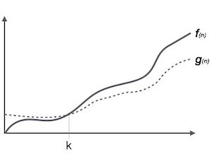
Fig: Big omega notation

Here, f (n) >= g (n)

Where n>=k and c>0, k>=1

If any algorithm satisfies the eq1 condition then it becomes f (n)= ῼ (g (n))

Consider the following example

In the above example g(n) is ‘2n’ and f(n) is ‘2n-2’ and value of constant is 0.5. The point where c*g(n) and f(n) intersect is ‘’n0’. Beyond ‘n0’ c*g(n) is always smaller than f(n) for constant ‘0.5’. We can write the conclusion as follows

f(n) = Ω g(n) for constant ‘c’ =0.5 and ‘n0’=2

Such that c*g(n)<= f(n) for all n>n0

Theta (Θ) Notation

• It is the formal way to express the time complexity.
• It is used to define the lower as well as upper bound of an algorithm’s running time.
• It shows the average case time complexity or average of time taken by the algorithm to perform a certain task.

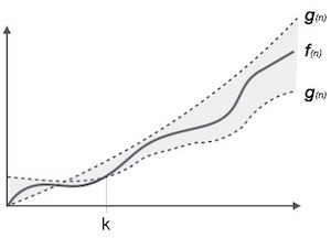
Fig: Theta notation

Let C1 g(n) be upper bound and C2 g(n) be lower bound.

C1 g(n)<= f (n)<=C2 g(n)

Where C1, C2>0 and n>=k

Consider the following example

In the above example g(n) is ‘2n’ and f(n) is ‘3n-2’ and value of constant c1 is 0.5 and c2 is 2. The point where c*g(n) and f(n) intersect is ‘’n0’. Beyond ‘n0’ c1*g(n) is always smaller than f(n) for constant ‘0.5’ and c2*g(n) is always greater than f(n) for constant ‘2’. We can write the conclusion as follows

f(n)=Ω g(n) for constant ‘c1’ =0.5, ‘c2’ = 2 and ‘n0’=2

Such that c1*g(n)<= f(n)<=c2*g(n) for all n>n0

Key takeaway

Big Oh is used to define the upper bound of an algorithm’s running time.

Big Omega is used to define the lower bound of an algorithm’s running time.

Theta is used to define the lower as well as upper bound of an algorithm’s running time.

1.4 Time-Space trade off

Complexity of an algorithm is the function which gives the running time and space requirement of an algorithm in terms of size of input data. Frequency count refers to the number of times particular instructions executed in a block of code. Frequency count plays important role in the performance analysis of an algorithm. Each instruction in algorithm is incremented by one as its execution. Frequency count analysis is the form of priori analysis. Frequency count analysis produces output in terms of time complexity and space complexity.

• Time complexity: Time complexity is about to number of times compiler execute basic operations in instruction. That is because basic operations are so defined that the time for the other operations is much less than or at most proportional to the time for the basic operations. To determine time complexity user need to calculate frequency count and express it in terms of notations. Total time taken by program is the summation of compile time and running time. Out of these two main point to take care about is running time as it depends upon the number and magnitude of input and output.
• Space complexity: Space complexity is about to maximum amount of memory required for algorithm. To determine space complexity user need to calculate frequency count and express it in terms of notations.

Frequency count analysis for this code is as follows

In the above example, for the first four instructions there is no frequency count. For data declaration and the inclusion of header file there is no frequency count. So, for this example has a frequency count for time is 2 and a frequency count for space is 1. So, total frequency count is 3.

Consider the following example

Explanation: In the above example, one is add to frequency count for instruction four and seven after that in fifth instruction is check from zero to five so it will add value six to frequency count. ‘For’ loop executed for five times so for  sixth instruction frequency count is five. Total frequency count for above program is 1+6+5+1 =13.

Consider the following example

Explanation: In the above example, in instruction five value of ‘i’ is check from 0 to ‘m’ so frequency count is ‘m+1’ for fifth instruction. In instruction five value of ‘j’ is check from 0 to ‘n’ so frequency count is ‘n+1’ but this instruction is in the for loop which execute for ‘m’ times, so for seventh instruction is m*(n+1). Ninth instruction is in the two for loops, out of which first for loop execute for m times and second ‘for’ loop execute for ‘n’ times. So for ninth instruction frequency count is m*n. The total frequency count for the above program is

(m+1)+m(n+1)+mn=2m+2mn+1=2m(1+n)+1.

Consider the following example

Explanation: For above program total frequency count

=(m+1)+m(n+1)+mn+mn(n+1)+mn

=m+1+mn+m+mn+mn2 +mn+mn2

=2 mn2+3mn+2m+1

=mn(2n+3)+2m+1

Consider the following example

Explanation: the above example, one is add to frequency count for instruction four. The loop will execute till value of n is incremented to 10 from 1, so for loop statements ie instructions seven and eight is execute for tem times. When the value of ‘n’ is ten then ‘break’ statement will execute for one time and it will skip the tenth execution of tenth instruction. Tenth instruction will add value nine to frequency count. Total frequency count for above program is 10+10+1+9+10 = 40.

1.5 Searching: Linear Search and Binary Search Techniques and their complexity analysis

Linear Search

A linear or sequential relationship exists when data objects are stored in a collection, such as a list. Each data item is kept in a certain location in relation to the others. These relative positions are the index values of the various items in Python lists. We can access these index values in order because their values are ordered. Our initial searching strategy, the sequential search, is born out of this procedure.

This is how the search works, as shown in the diagram. We just advance from item to item in the list, following the underlying sequential ordering, until we either find what we're looking for or run out of options. If we run out of items, we have discovered that the item we were searching for was not present.

Fig: Sequential search

Algorithm

●      LINEAR_SEARCH(A, N, VAL)

●      Step 1: [INITIALIZE] SET POS = -1

●      Step 2: [INITIALIZE] SET I = 1

●      Step 3: Repeat Step 4 while I<=N

●      Step 4: IF A[I] = VAL

SET POS = I

PRINT POS

Go to Step 6

[END OF IF]

SET I = I + 1

[END OF LOOP]

●      Step 5: IF POS = -1

PRINT " VALUE IS NOT PRESENTIN THE ARRAY "

[END OF IF]

●      Step 6: EXIT

Function for Linear search is

Find(values, target)

{

For( i = 0; i < values.length; i++)

 {

If (values[i] == target)

{ return i; }

}

Return –1;

}

If an element is found this function returns the index of that element otherwise it returns –1.

Example: we have an array of integers, like the following:

Let’s search for the number 7. According to function for linear search index for element 7 should be returned. We start at the beginning and check the first element in the array.

First element is 9. Match is not found and hence we move to next element i.e., 6.

Again, match is not found so move to next element i.e.,7.

We found the match at the index position 2. Hence output is 2.

If we try to find element 10 in above array, it will return –1, as 10 is not present in the array.

Complexity Analysis of Linear Search:

Let us assume element x is to be searched in array A of size n.

An algorithm can be analyzed using the following three cases.

1. Worst case

2. Average case

3. Best case

1. Worst case: In Linear search worst case happens when element to be searched is not present. When x is not present, the linear search function compares it with all the elements of A one by one. The size of A is n and hence x is to be compared with all n elements. Thus, the worst-case time complexity of linear search would be O(n).

2. Average case: In average case analysis, we take all possible inputs and calculate computing time for all of the inputs. Sum all the calculated values and divide the sum by total number of inputs. Following is the value of average case time complexity.

Average Case Time=∑=  ×=O (n)

3. Best Case: In linear search, the best case occurs when x is present at the first location. So, time complexity in the best-case would-be O (1).

P: Program for Linear Search

#include<stdio.h>

#include<conio.h>

Int search(int [],int, int);

Void main()

{
int a[20],k,i,n,m;

Clrscr();

Printf(“\n\n ENTER THE SIZE OF ARRAY”);

Scanf(“%d”,&n);

Printf(“\n\nENTER THE ARRAY ELEMENTS\n\n”);

For(i=0;i<n;i++)
{
scanf(“%d”,&a[i]);
}
printf(“\n\nENTER THE ELEMENT FOR SEARCH\n”);
scanf(“%d”,&k);
m=search(a,n,k);
if(m==–1)
{
printf(“\n\nELEMENT IS NOT FOUND IN LIST”);
}
else
{
printf(“\n\nELEMENT IS FOUND AT LOCATION %d”,m);
}
}
getch();
}

Int search(int a[],int n,int k)
{
int i;
for(i=0;i<n;i++)
{
if(a[i]==k)
{
return i;
}
}
if(i==n)
{
return –1;
}

}

Merits:

1. Simple and easy to implement
2. It works well even on unsorted arrays.
3. It is memory efficient as it does not require copying and partitioning of the array being searched.

Demerits:

1. Suitable only for small number of values.
2. It is slow as compared to binary search.

Binary Search

Binary search is the search technique which works efficiently on the sorted lists. Hence, in order to search an element into some list by using binary search technique, we must ensure that the list is sorted.

Binary search follows a divide and conquer approach in which the list is divided into two halves and the item is compared with the middle element of the list. If the match is found then, the location of the middle element is returned; otherwise, we search into either of the halves depending upon the result produced through the match.

Binary search algorithm is given below.

BINARY_SEARCH(A, lower_bound, upper_bound, VAL)

Step 1: [INITIALIZE] SET BEG = lower_bound

END = upper_bound, POS = - 1

Step 2: Repeat Steps 3 and 4 while BEG <=END

Step 3: SET MID = (BEG + END)/2

Step 4: IF A[MID] = VAL

SET POS = MID

PRINT POS

Go to Step 6

ELSE IF A[MID] > VAL

SET END = MID – 1

ELSE

SET BEG = MID + 1

[END OF IF]

[END OF LOOP]

Step 5: IF POS = -1

PRINT "VALUE IS NOT PRESENT IN THE ARRAY"

[END OF IF]

Step 6: EXIT

Complexity

Example 1:

Let us consider an array arr = {1, 5, 7, 8, 13, 19, 20, 23, 29}. Find the location of the item 23 in the array.

In 1st step:

1. BEG = 0  
2. END = 8ron 
3. MID = 4  
4. a[mid] = a[4] = 13 < 23, therefore 

In Second step:

1. Beg = mid +1 = 5  
2. End = 8 
3. Mid = 13/2 = 6   
4. a[mid] = a[6] = 20 < 23, therefore;  

In third step:

1. Beg = mid + 1 = 7  
2. End = 8  
3. Mid = 15/2 = 7 
4. a[mid] = a[7]  
5. a[7] = 23 = item;  
6. Therefore, set location = mid;  
7. The location of the item will be 7.  

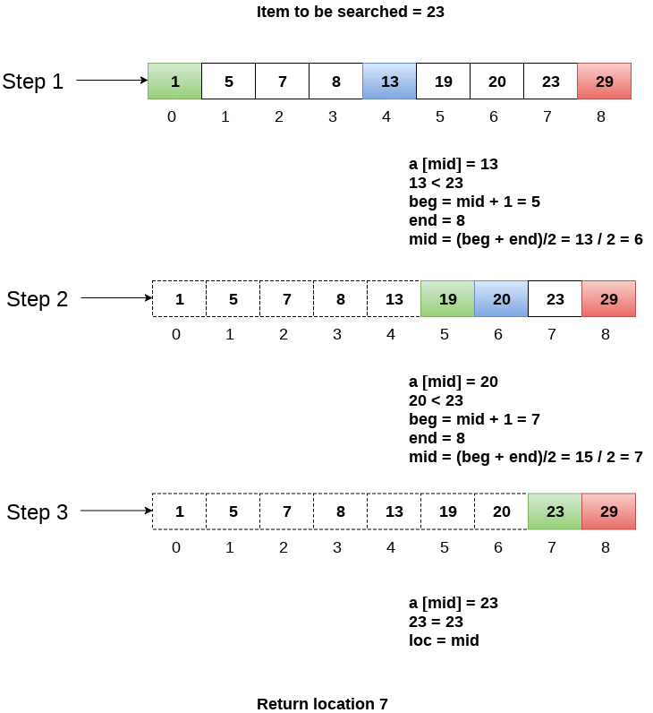
Fig- Example

Example 2: Find 103 in {–1, 5, 6, 18, 19, 25, 46, 78, 102, 114} using Binary Search.

Step 1: Low=0

High=9

Step 2: Mid=(0+9)/2=4

So middle element is 19.

Step 3: Compare(103,19)

103>19 hence element is located at right half of array and we can ignore left half of array. Update Low and recalculate mid.

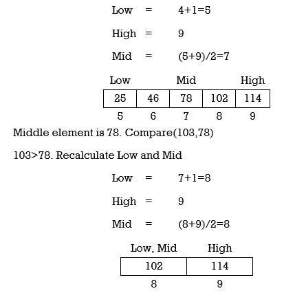
Middle element is 102. Compare(103,102)

103>102. Recalculate Low and Mid.

Low=8+1=9

High=9

Here Low=High and match is not found hence we conclude that element is not present in array.

Example 3: Find 44 in A={5,12,17,23,38,44,77,84,90} using binary search.

Step 1:Low=0

High=8

Mid=(0+8)/2=4

Middle element is 38. Compare(44,38)

44>38.Thus element is located at right half of array and we can ignore left half of array. Recalculate Low and Mid.

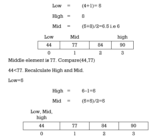
Middle element is 44. Compare(44,44)

Match is Found. Return index and print “Element Found.”

Algorithm for Recursive Binary Search

Int BinarySearch (int A[], int x, int Low, int High)

{

If (High > Low)

Return –1;

Int mid = (High + Low) / 2;

If (A[mid] == x)

Return mid;

If (A[mid] < x)

Return BinarySearch(A, x, mid+1, High);

Return BinarySearch(A, x, Low, mid–1);

}

Program for Binary Search

#include<stdio.h>

#include<conio.h>

Void main()

{

Int n,i,search,f=0,low,high,mid,a[20];

Clrscr();

Printf("Enter the number of elements:");

Scanf("%d",&n);

For(i=1;i<=n;i++)

{

Printf("Enter the number in ascending order a[%d]=",i);

Scanf("%d",&a[i]);

}

Printf("Enter the element to be searched:");

Scanf("%d",&search);

Low=0;

High=n–1;

While(low<=high)

{

Mid=(low+high)/2;

If(search<a[mid])

{

High=mid–1;

}

Else if(search>a[mid])

{

Low=mid+1;

}

Else

{

f=1;

Printf("Element is found at the position %d:",mid);

Exit();

}

}

If(f==0)

{

Printf("Element not found");

}

Getch();

}

Merits:

Binary Search is fast and efficient.

Suitable for large number of values.

Demerits:

Binary search works only on sorted array or list.

References:

1. Horowitz and Sahani, “Fundamentals of Data Structures”, Galgotia Publications Pvt Ltd Delhi India.
2. Lipschutz, “Data Structures” Schaum’s Outline Series, Tata McGraw-hill Education (India) Pvt. Ltd.
3. Thareja, “Data Structure Using C” Oxford Higher Education.
4. AK Sharma, “Data Structure Using C”, Pearson Education India.