Unit - 4

Trees

4.1 Basic Tree Terminologies

Introduction

A tree data structure can be defined recursively (locally) as a collection of nodes (starting at a root node), where each node is a data structure consisting of a value, together with a list of references to nodes (the "children"), with the constraints that no reference is duplicated, and none points to the root.

Definition of TREE:

A tree is defined as a set of one or more nodes T such that:

There is a specially designed node called root node

The remaining nodes are partitioned into N disjoint set of nodes T1, T2,…..Tn, each of which is a tree.

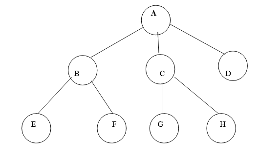
Fig. Example of tree

In above tree A is Root.

Remaining nodes are partitioned into three disjoint sets:

{B, E, F}, {C, G, H}, {D}.

All these sets satisfies the properties of tree.

Some examples of TREE and NOT TREE

  Each linear list is trivially a tree

    Not a tree: cycle A→A

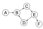  Not a tree: cycle B→C→E→D→B

  Not a tree: two non-(connected parts, A→B and C→D→E

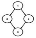Not a tree: undirected cycle 1-2-4-3

Fig. Examples of tree and no tree

Tree Terminologies

1. Root – The top node in a tree.
2. Parent – The converse notion of child.
3. Siblings – Nodes with the same parent.
4. Descendant – a node reachable by repeated proceeding from parent to child.
5. Ancestor – a node reachable by repeated proceeding from child to parent.
6. Leaf – a node with no children.
7. Internal node – a node with at least one child.
8. External node – a node with no children.
9. Degree – number of sub trees of a node.
10. Edge – connection between one node to another.
11. Path – a sequence of nodes and edges connecting a node with a descendant.
12. Level – The level of a node is defined by 1 + the number of connections between the node and the root.
13. Height of tree –The height of a tree is the number of edges on the longest downward path between the root and a leaf.
14. Height of node –The height of a node is the number of edges on the longest downward path between that node and a leaf.
15. Depth –The depth of a node is the number of edges from the node to the tree's root node.
16. Forest – A forest is a set of n ≥ 0 disjoint trees.

4.2 Different types of Trees: Binary Tree, Threaded Binary Tree, Binary Search Tree, AVL Tree

Binary Tree

A binary tree is a special case of tree in which no node of a tree can have degree more than two.

Definition of Binary Tree:

A binary tree is made of nodes, where each node contains a "left" pointer, a "right" pointer, and a data element. The "root" pointer points to the topmost node in the tree. The left and right pointers recursively point to smaller "subtrees" on either side. A null pointer represents a binary tree with no elements -- the empty tree.

The formal recursive definition is A binary tree is either empty (represented by a null pointer), or is made of a single node, where the left and right pointers (recursive definition ahead) each point to a binary tree.

Example of Binary Tree:

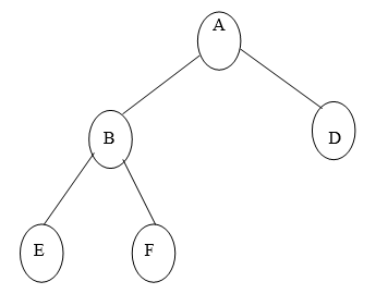
Fig. Example of Binary Tree

Types of Binary Tree,

1. Left Skewed Binary Tree:

2. Right Skewed Binary Tree:

1. Left Skewed Binary Tree:

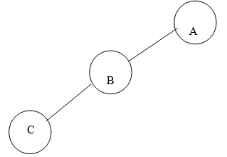
Fig.  Example of Left Skewed Binary Tree

In this tree, every node is having only Left sub tree.

2. Right Skewed Binary Tree:

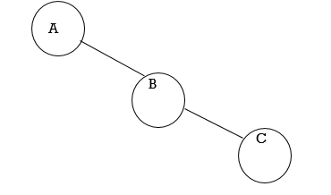
Fig. Example of Right Skewed Binary Tree

In this tree, every node is having only Right sub tree.

Full or strict Binary Tree:

It is a binary tree of depth K having 2k-1 nodes.

For k=3, number of nodes=7

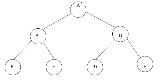
Fig. Example of strict Binary Tree

Complete Binary Tree:

It is a binary tree of depth K with N nodes in which these N nodes can be numbered sequentially from 1 to N.

Since a binary tree is an ordered tree and has levels, it is convenient to assign a number to each node.

Suppose for K=3:

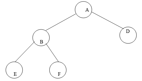
Fig. Example of Complete Binary Tree

The nodes can be numbered sequentially like:

Fig. Representation of Complete Binary Tree

Consider another example of binary tree:

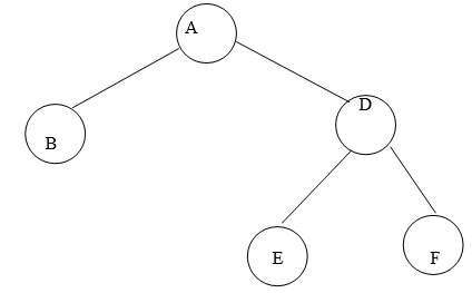
Fig. Example of Non Complete Binary Tree

If we try to give numbers to nodes it would appear like:

Fig. Representation of Non Complete Binary Tree

Here nodes cannot be numbers sequentially, so this kind of tree cannot be called as a complete binary tree

Binary Search Tree

We now turn our attention to search tress: Binary Search tress in this chapter and AVL Trees in next chapter. As seen in previous chapter, the array structure provides a very efficient search algorithm, the binary search, but it is inefficient for insertion and deletion algorithms. On the other hand, linked list structure provides efficient insertion and deletion algorithms but it is very inefficient for search algorithm. So what we need is a structure that provides efficient insertion, deletion as well as search algorithms.

Basic Concept:

A Binary Search Tree is a binary tree with the following properties:

1. It may be empty and every node has an identifier.

2. All nodes in left subtree are less than the root.

2. All nodes in right subtree are greater than the root.

4. Each subtree is itself a BST.

Examples of BST:

Valid BSTs:

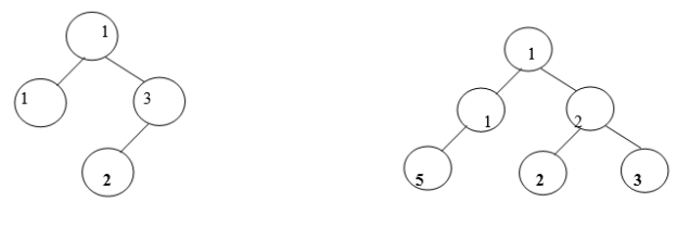
Fig. Examples of Valid BSTs

Invalid BSTs:

Fig. Examples of Invalid BSTs

Examine the BSTs in Fig.4.2. The first tree, Fig.4.2 (a) breaks the second rule: The left node 30 is greater than that of its root node 20. The second tree, Fig.4.2 (b) breaks the third rule: The right node 20 is less than that of its root node 50. The third tree, Fig.4.2 (c) breaks the second rule: The left node 25 is greater than that of its root node 10. It also breaks the third rule: The right node 08 is less than that of its root node 15.

Threaded Binary Tree

Binary trees, including binary search trees and their variants, can be used to store a set of items in a particular order. For example, a binary search tree assumes data items are ordered and maintain this ordering as part of their insertion and deletion algorithms. One useful operation on such a tree is traversal: visiting the items in the order in which they are stored .A simple recursive traversal algorithm that visits each node of a BST is the following. Assume t is a pointer to a node, or NULL.

       Algorithm traverse_tree (root):

       Input: a pointer root to a node (or NULL.)

                     If root = NULL, return.

                     Else

                          traverse_tree (left-child (root))

                          Visit t

                          traverse_tree (right-child (root))

The problem with this algorithm is that, because of its recursion, it uses stack space proportional to the height of a tree. If the tree is fairly balanced, this amounts to O(log n) space for a tree containing n elements.

One of the solutions to this problem is tree threading.

A threaded binary tree defined as follows:

"A binary tree is threaded by making all right child pointers that would normally be null point to the inorder successor of the node (if it exists), and all left child pointers that would normally be null point to the inorder predecessor of the node."

It is also possible to discover the parent of a node from a threaded binary tree, without explicit use of parent pointers or a stack. This can be useful where stack space is limited, or where a stack of parent pointers is unavailable (for finding the parent pointer via DFS).

Inorder Threaded Binary Tree:

In inorder threaded binary tree, left thread points to the predecessor and right thread points to the successor.

 Types Inorder Threaded Binary Tree:

• Right Inorder Threaded Binary Tree.

In this type of TBT, only right threads are shown which points to the successor.

• Left Inorder Threaded Binary Tree.

In this type of TBT, only left threads are shown which points to the predecessor.

For TBT it is not necessary that the tree must be BST, it can be applied to general tree.

Example: Draw inorder TBT for following data:

10,  8, 1 5, 7,  9, 12, 18

Solution:

Step 1: The general for given data is:

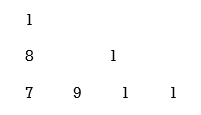
Step 2: Write inorder sequence for the above tree:

7, 8, 9, 10, 12, 15, 18

Step 3: Make groups containing three nodes per group like:

Step 4: It means right thread of 7 point to 8 provided that 7 node is not having right link, means right link of 7 is NULL and thread is pointing in bottom-up direction and not in top to bottom .

Left thread of 7 and Right thread of 18 will point to head node.

Step 5: Draw TBT with right and left threads.

  Head Node

Left Inorder Threaded Binary Tree:

Right Inorder Threaded Binary Tree:

AVL Trees (Adelsion Velski & Landis):

The concept is developed by three persons: Adelsion, Velski and Landis.

Balance Factor:

Balance factor is (Height of left sub tree - Height of right sub tree)

Height Balance Tree:

An empty tree is height balanced. If T is non empty binary tree with TL and TR as left and right sub tress, then T is height balanced if and only if:

TL and TR are height balanced.

HL- HR =1

HL  and   HR are heights of left and right sub tree.

For ant node in AVL tree Balance factor must be -1 or 0 or 1.

Following rotations are performed on AVL tree if any of the nodes is unbalanced.

1. LL Rotation.

2. LR Rotation.

3. RL Rotation.

4. RR Rotation.

1. LL Rotation:

Count from unbalanced node. First left node becomes the root node.

2. LR Rotation:

Count from unbalanced node. Go for left node and then right node say X.  The  node  X becomes the root node.

3. RL Rotation:

Count from unbalanced node. Go for right node and then left node say X.  The  node  X becomes the root node.

4. RR Rotation:

Count from unbalanced node. First right node becomes the root node.

While inserting data in AVL tree,  Follow the property of Binary search tree (left<root<right)

Example: obtain an AVL tree by inserting one integer at a time in following sequence:

150,155,160,115,110,140,120,145,130

SOLUTION:

Step 1: insert 150

150

Balance factor for 150 is: 0 – 0=0

1500

NO ROTATION IS REQUIRED.

Step 2: insert 155

Balance factor for 150 is: 0 – 1= -1

Both nodes are balanced.

NO ROATION IS REQIURED.

STEP 3: INSERT 160.

Balance factor of 150 is -2. So 150 is unbalanced. Some rotation is required to do 150 as balanced node.  Start from 150 towards 160.

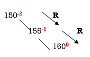
We get RR direction. So we have to perform RR rotation.

In RR rotation, Count from unbalanced node. First right node becomes the root node. So here first R is 155. So 155 will become the root.

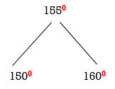
Now all nodes are balanced.

STEP 4: INSERT 115.

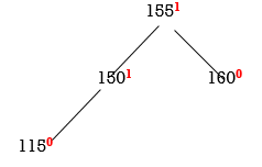
All nodes are balanced. NO ROTATION IS REQUIRED.

STEP 5: INSERT 110

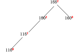
155 and 150 are unbalanced. Whenever two/more nodes are unbalanced, we have to consider the lowermost node first. i.e.150. Move from 150 towards the node causing unbalancing (110)

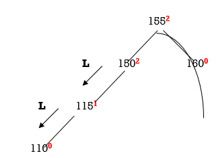
So we have to perform LL Rotation. In LL rotation, Count from unbalanced node. First Left node becomes the root node. So here first L is 115. So 115 will become the root.

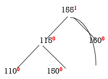
Now all nodes are balanced.

STEP 6: INSERT 140  

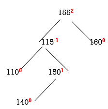
155 is unbalanced. Count move from 155 towards the node causing unbalancing (140).

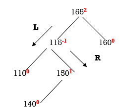
So we have to perform LR Rotation. In LR rotation, Count from unbalanced node(155). Go for left node and then right node (150).  150 will become root node

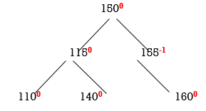
Now all nodes are balanced.

STEP 7: INSERT 120

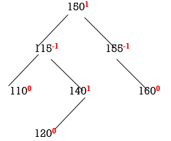
Now all nodes are balanced.

STEP 8: INSERT 145

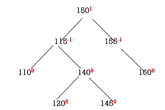
Now all nodes are balanced.

STEP 9: INSERT 130

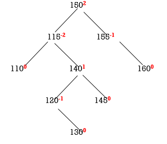
Two nodes 150 and 115 are unbalanced. First consider 115. Count move from 115 towards the node causing unbalancing (130).

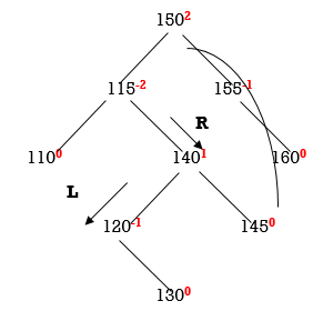
So we have to perform RL Rotation. In RL rotation, Count from unbalanced node(115). Go for Right node and then Left node (120).  120 will become root node.

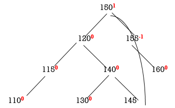
Now all nodes are balanced.

Thus the tree is balanced.

4.3 Tree operations on each of the trees and their algorithms with complexity analysis

Following are the basic operations of a tree −

Search − Searches an element in a tree.

Insert − Inserts an element in a tree.

Pre-order Traversal − Traverses a tree in a pre-order manner.

In-order Traversal − Traverses a tree in an in-order manner.

Post-order Traversal − Traverses a tree in a post-order manner.

Node

Define a node having some data, references to its left and right child nodes.

Struct node {

   int data;  

   struct node *leftChild;

   struct node *rightChild;

};

Search Operation

Whenever an element is to be searched, start searching from the root node. Then if the data is less than the key value, search for the element in the left subtree. Otherwise, search for the element in the right subtree. Follow the same algorithm for each node.

Algorithm

Struct node* search(int data){

   struct node *current = root;

   printf("Visiting elements: ");

   while(current->data != data){

      if(current != NULL) {

         printf("%d ",current->data);

         //go to left tree

         if(current->data > data){

            current = current->leftChild;

         }  //else go to right tree

         else {               

            current = current->rightChild;

         }

         //not found

         if(current == NULL){

            return NULL;

         }

      }

   }

   return current;

}

Insert Operation

Whenever an element is to be inserted, first locate its proper location. Start searching from the root node, then if the data is less than the key value, search for the empty location in the left subtree and insert the data. Otherwise, search for the empty location in the right subtree and insert the data.

Algorithm

Void insert(int data) {

   struct node *tempNode = (struct node*) malloc(sizeof(struct node));

   struct node *current;

   struct node *parent;

   tempNode->data = data;

   tempNode->leftChild = NULL;

   tempNode->rightChild = NULL;

   //if tree is empty

   if(root == NULL) {

      root = tempNode;

   } else {

      current = root;

      parent = NULL;

      while(1) {               

         parent = current;

         //go to left of the tree

         if(data < parent->data) {

            current = current->leftChild;               

            //insert to the left

            if(current == NULL) {

               parent->leftChild = tempNode;

               return;

            }

         }  //go to right of the tree

         else {

            current = current->rightChild;

            //insert to the right

            if(current == NULL) {

               parent->rightChild = tempNode;

               return;

            }

         }

      }           

   }

}  

4.4 Applications of Binary Trees

Huffman’s Algorithm:

Huffman Codes:

Huffman coding is a simple data compression scheme.

Fixed-Length Codes

Suppose we want to compress a 100,000-byte data file that we know contains only the lowercase letters A through F. Since we have only six distinct characters to encode, we can represent each one with three bits rather than the eight bits normally used to store characters:

This fixed-length code gives us a compression ratio of 5/8 = 62.5%.

Variable-Length Codes

What if we knew the relative frequencies at which each letter occurred? It would be logical to assign shorter codes to the most frequent letters and save longer codes for the infrequent letters. For example, consider this code:

Using this code, our file can be represented with

(45×1 + 13×3 + 12×3 + 16×3 + 9×4 + 5×4) × 1000 = 224 000 bits

Or 28 000 bytes, which gives a compression ratio of 72%. In fact, this is an optimal character code for this file (which is not to say that the file is not further compressible by other means).

Prefix Codes

Notice that in our variable-length code, no codeword is a prefix of any other codeword. For example, we have a codeword 0, so no other codeword starts with 0. And both of our four-bit code words start with 110, which is not a codeword. Such codes are called prefix codes. Prefix codes are useful because they make a stream of bits unambiguous; we simply can accumulate bits from a stream until we have completed a codeword. (Notice that encoding is simple regardless of whether our code is a prefix code: we just build a dictionary of letters to code words, look up each letter we're trying to encode, and append the code words to an output stream.) In turns out that prefix codes always can be used to achieve the optimal compression for a character code, so we're not losing anything by restricting ourselves to this type of character code.

When we're decoding a stream of bits using a prefix code, what data structure might we want to use to help us determine whether we've read a whole codeword yet?

One convenient representation is to use a binary tree with the code words stored in the leaves so that the bits determine the path to the leaf. In our example, the codeword 1100 is found by starting at the root, moving down the right sub tree twice and the left sub tree twice.

Huffman’s algorithm is used to build such type of binary tree.

Algorithm:

Arrange list in ascending order of frequencies.

Create new node with addition of frequencies of first two nodes.

Insert this new node into list and again sort it.

Repeat till only one value remains in the list.

Consider alphabets and their frequencies of occurrences are as:

Huffman Algorithm for above data will work like:

Step1: Sort the list in ascending order

Step2: New node’s frequency=5+9=14

Step3: New node’s frequency=12+13=25

14162545

Step4: New node’s frequency=14+16=30

Step5: New node’s frequency=25+30=55

Step6: New node’s frequency=45+55=100

Final Huffman’s tree will be:

4.5 B Tree, B+ Tree: definitions, algorithms and analysis

Introduction to B-Trees

A B-tree is a tree data structure that keeps data sorted and allows searches, insertions, and deletions in logarithmic amortized time. Unlike self-balancing binary search trees, it is optimized for systems that read and write large blocks of data. It is most commonly used in database and file systems.

The B-Tree Rules

Important properties of a B-tree:

B-tree nodes have many more than two children.

A B-tree node may contain more than just a single element.

The set formulation of the B-tree rules: Every B-tree depends on a positive constant integer called MINIMUM, which is used to determine how many elements are held in a single node.

Rule 1: The root can have as few as one element (or even no elements if it also has no children); every other node has at least MINIMUM elements.

Rule 2: The maximum number of elements in a node is twice the value of MINIMUM.

Rule 3: The elements of each B-tree node are stored in a partially filled array, sorted from the smallest element (at index 0) to the largest element (at the final used position of the array).

Rule 4: The number of subtrees below a nonleaf node is always one more than the number of elements in the node.

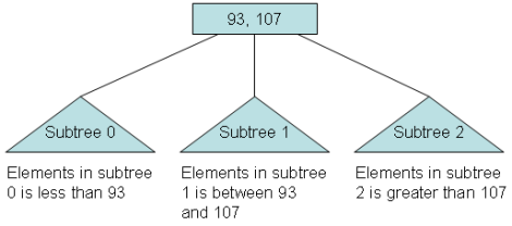
Subtree 0, subtree 1, ...

Rule 5: For any nonleaf node:

An element at index i is greater than all the elements in subtree number i of the node, and

An element at index i is less than all the elements in subtree number i + 1 of the node.

Rule 6: Every leaf in a B-tree has the same depth. Thus it ensures that a B-tree avoids  the problem of a unbalanced tree.

B+-trees

Most queries can be executed more quickly if the values are stored in order. But it's not practical to hope to store all the rows in the table one after another, in sorted order, because this requires rewriting the entire table with each insertion or deletion of a row.

This leads us to instead imagine storing our rows in a tree structure. Our first instinct would be a balanced binary search tree like a red-black tree, but this really doesn't make much sense for a database since it is stored on disk. You see, disks work by reading and writing whole blocks of data at once — typically 512 bytes or four kilobytes. A node of a binary search tree uses a small fraction of that, so it makes sense to look for a structure that fits more neatly into a disk block.

Hence the B+-tree, in which each node stores up to d references to children and up to d − 1 keys. Each reference is considered “between” two of the node's keys; it references the root of a subtree for which all values are between these two keys.

Here is a fairly small tree using 4 as our value for d.

A B+-tree requires that each leaf be the same distance from the root, as in this picture, where searching for any of the 11 values (all listed on the bottom level) will involve loading three nodes from the disk (the root block, a second-level block, and a leaf).

In practice, d will be larger — as large, in fact, as it takes to fill a disk block. Suppose a block is 4KB, our keys are 4-byte integers, and each reference is a 6-byte file offset. Then we'd choose d to be the largest value so that 4 (d − 1) + 6 d ≤ 4096; solving this inequality for d, we end up with d ≤ 410, so we'd use 410 for d. As you can see, d can be large.

A B+-tree maintains the following invariants:

Every node has one more references than it has keys.

All leaves are at the same distance from the root.

For every non-leaf node N with k being the number of keys in N: all keys in the first child's subtree are less than N's first key; and all keys in the ith child's subtree (2 ≤ i ≤ k) are between the (i − 1)th key of n and the ith key of n.

The root has at least two children.

Every non-leaf, non-root node has at least floor(d / 2) children.

Each leaf contains at least floor(d / 2) keys.

Every key from the table appears in a leaf, in left-to-right sorted order.

In our examples, we'll continue to use 4 for d. Looking at our invariants, this requires that each leaf have at least two keys, and each internal node to have at least two children (and thus at least one key).

Insertion algorithm

Descend to the leaf where the key fits.

If the node has an empty space, insert the key/reference pair into the node.

If the node is already full, split it into two nodes, distributing the keys evenly between the two nodes. If the node is a leaf, take a copy of the minimum value in the second of these two nodes and repeat this insertion algorithm to insert it into the parent node. If the node is a non-leaf, exclude the middle value during the split and repeat this insertion algorithm to insert this excluded value into the parent node.

Initial: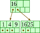
Insert 20: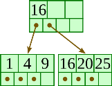
Insert 13: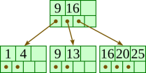
Insert 15: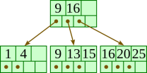
Insert 10: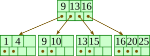
Insert 11: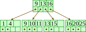
Insert 12:

Deletion algorithm

Descend to the leaf where the key exists.

Remove the required key and associated reference from the node.

If the node still has enough keys and references to satisfy the invariants, stop.

If the node has too few keys to satisfy the invariants, but its next oldest or next youngest sibling at the same level has more than necessary, distribute the keys between this node and the neighbor. Repair the keys in the level above to represent that these nodes now have a different “split point” between them; this involves simply changing a key in the levels above, without deletion or insertion.

If the node has too few keys to satisfy the invariant, and the next oldest or next youngest sibling is at the minimum for the invariant, then merge the node with its sibling; if the node is a non-leaf, we will need to incorporate the “split key” from the parent into our merging. In either case, we will need to repeat the removal algorithm on the parent node to remove the “split key” that previously separated these merged nodes — unless the parent is the root and we are removing the final key from the root, in which case the merged node becomes the new root (and the tree has become one level shorter than before).

Initial: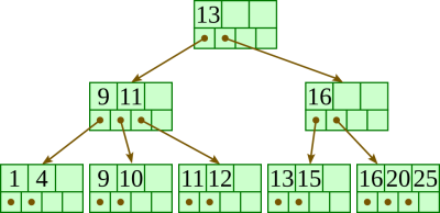
Delete 13: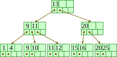
Delete 15: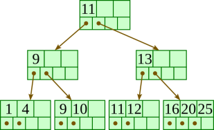
Delete 1: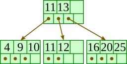

4.6 Binary Heaps

A binary heap is a data structure that resembles a complete binary tree in appearance. The ordering features of the heap data structure are explained here. A Heap is often represented by an array. We'll use H to represent a heap.

Because the elements of a heap are kept in an array, the position of the parent node of the ith element can be located at i/2 if the starting index is 1. Position 2i and 2i + 1 are the left and right children of the ith node, respectively.

Based on the ordering property, a binary heap can be classed as a max-heap or a min-heap.

Max Heap

A node's key value is larger than or equal to the key value of the highest child in this heap.

Hence, H[Parent(i)] ≥ H[i]

Fig: Max heap

Max Heap Construction Algorithm

The technique for creating Min Heap is similar to that for creating Max Heap, only we use min values instead of max values.

By inserting one element at a time, we will derive a method for max heap. The property of a heap must be maintained at all times. We also presume that we are inserting a node into an already heapify tree while inserting.

Step 1: Make a new node at the bottom of the heap.

Step 2: Give the node a new value.

Step 3: Compare this child node's value to that of its parent.

Step 4: If the parent's value is smaller than the child's, swap them.

Step 5: Repeat steps 3 and 4 until the Heap property is maintained.

Min Heap

In mean-heap, a node's key value is less than or equal to the lowest child's key value.

Hence, H[Parent(i)] ≤ H[i]

Basic operations with respect to Max-Heap are shown below in this context. The insertion and deletion of elements in and out of heaps necessitates element reordering. As a result, the Heapify function must be used.

Fig: Min heap

Max Heap Deletion Algorithm

Let's create an algorithm for deleting from the maximum heap. The root of the Max (or Min) Heap is always deleted to remove the maximum (or minimum) value.

Step 1: Remove the root node first.

Step 2: Move the last element from the previous level to the root.

Step 3: Compare this child node's value to that of its parent.

Step 4: If the parent's value is smaller than the child's, swap them.

Step 5: Repeat steps 3 and 4 until the Heap property is maintained.

Key takeaway

The ordering features of the heap data structure are explained here. A Heap is often represented by an array.

References:

1. Algorithms, Data Structures, and Problem Solving with C++”, Illustrated Edition by Mark Allen Weiss, Addison-Wesley Publishing Company.

2. “How to Solve it by Computer”, 2nd Impression by R.G. Dromey, Pearson Education.

3. “Fundamentals of Data Structures”, Illustrated Edition by Ellis Horowitz, Sartaj Sahni, Computer Science Press.