Unit - 5
Graphs
A graph can be defined as group of vertices and edges that are used to connect these vertices. A graph can be seen as a cyclic tree, where the vertices (Nodes) maintain any complex relationship among them instead of having parent child relationship.
Definition
A graph G can be defined as an ordered set G (V, E) where V(G) represents the set of vertices and E(G) represents the set of edges which are used to connect these vertices.
Example
The following is a graph with 5 vertices and 6 edges.
This graph G can be defined as G = (V, E)
Where V = {A, B, C, D, E} and E = {(A, B), (A, C) (A, D), (B, D), (C, D), (B, E), (E, D)}.

Directed and Undirected Graph
A graph can be directed or undirected. However, in an undirected graph, edges are not associated with the directions with them. An undirected graph is shown in the above figure since its edges are not attached with any of the directions. If an edge exists between vertex A and B then the vertices can be traversed from B to A as well as A to B.
In a directed graph, edges form an ordered pair. Edges represent a specific path from some vertex A to another vertex B. Node A is called the initial node while node B is called terminal node.
A directed graph is shown in the following figure.
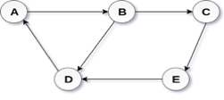
Fig– Directed graph
Graph Terminology
We use the following terms in graph data structure.
Vertex
Individual data element of a graph is called as Vertex. Vertex is also known as node. In above example graph, A, B, C, D & E are known as vertices.
Edge
An edge is a connecting link between two vertices. Edge is also known as Arc. An edge is represented as (startingVertex, endingVertex). For example, in above graph the link between vertices A and B is represented as (A, B). In above example graph, there are 7 edges (i.e., (A, B), (A, C), (A, D), (B, D), (B, E), (C, D), (D, E)).
Edges are three types.
- Undirected Edge - An undirected edge is a bidirectional edge. If there is undirected edge between vertices A and B then edge (A, B) is equal to edge (B, A).
- Directed Edge - A directed edge is a unidirectional edge. If there is directed edge between vertices A and B then edge (A, B) is not equal to edge (B, A).
- Weighted Edge - A weighted edge is an edge with value (cost) on it.
Undirected Graph
A graph with only undirected edges is said to be undirected graph.
Directed Graph
A graph with only directed edges is said to be directed graph.
Mixed Graph
A graph with both undirected and directed edges is said to be mixed graph.
End vertices or Endpoints
The two vertices joined by edge are called end vertices (or endpoints) of that edge.
Origin
If an edge is directed, its first endpoint is said to be the origin of it.
Destination
If an edge is directed, its first endpoint is said to be the origin of it and the other endpoint is said to be the destination of that edge.
Adjacent
If there is an edge between vertices A and B then both A and B are said to be adjacent. In other words, vertices A and B are said to be adjacent if there is an edge between them.
Incident
Edge is said to be incident on a vertex if the vertex is one of the endpoints of that edge.
Outgoing Edge
A directed edge is said to be outgoing edge on its origin vertex.
Incoming Edge
A directed edge is said to be incoming edge on its destination vertex.
Degree
Total number of edges connected to a vertex is said to be degree of that vertex.
Indegree
Total number of incoming edges connected to a vertex is said to be indegree of that vertex.
Outdegree
Total number of outgoing edges connected to a vertex is said to be outdegree of that vertex.
Parallel edges or Multiple edges
If there are two undirected edges with same end vertices and two directed edges with same origin and destination, such edges are called parallel edges or multiple edges.
Self-loop
Edge (undirected or directed) is a self-loop if its two endpoints coincide with each other.
Simple Graph
A graph is said to be simple if there are no parallel and self-loop edges.
Path
A path is a sequence of alternate vertices and edges that starts at a vertex and ends at other vertex such that each edge is incident to its predecessor and successor vertex.
Graph Representation
By Graph representation, we simply mean the technique which is to be used in order to store some graph into the computer's memory.
There are two ways to store Graph into the computer's memory.
1. Sequential Representation
In sequential representation, we use an adjacency matrix to store the mapping represented by vertices and edges. In adjacency matrix, the rows and columns are represented by the graph vertices. A graph having n vertices, will have a dimension n x n.
An entry Mij in the adjacency matrix representation of an undirected graph G will be 1 if there exists an edge between Vi and Vj.
An undirected graph and its adjacency matrix representation is shown in the following figure.
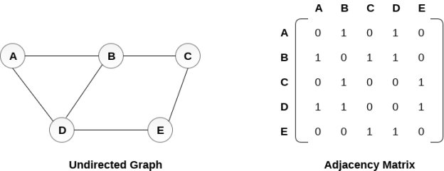
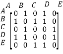

Fig: Undirected graph and its adjacency matrix
In the above figure, we can see the mapping among the vertices (A, B, C, D, E) is represented by using the adjacency matrix which is also shown in the figure.
There exists different adjacency matrices for the directed and undirected graph. In directed graph, an entry Aij will be 1 only when there is an edge directed from Vi to Vj.
A directed graph and its adjacency matrix representation is shown in the following figure.

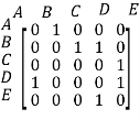

Fig- Directed graph and its adjacency matrix
Representation of weighted directed graph is different. Instead of filling the entry by 1, the Non-zero entries of the adjacency matrix are represented by the weight of respective edges.
The weighted directed graph along with the adjacency matrix representation is shown in the following figure.
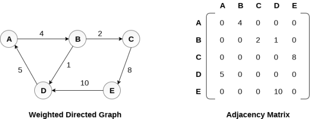

Fig - Weighted directed graph
2. Linked Representation
In the linked representation, an adjacency list is used to store the Graph into the computer's memory.
Consider the undirected graph shown in the following figure and check the adjacency list representation.

An adjacency list is maintained for each node present in the graph which stores the node value and a pointer to the next adjacent node to the respective node. If all the adjacent nodes are traversed then store the NULL in the pointer field of last node of the list. The sum of the lengths of adjacency lists is equal to the twice of the number of edges present in an undirected graph.
Consider the directed graph shown in the following figure and check the adjacency list representation of the graph.
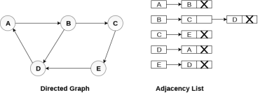
In a directed graph, the sum of lengths of all the adjacency lists is equal to the number of edges present in the graph.
In the case of weighted directed graph, each node contains an extra field that is called the weight of the node. The adjacency list representation of a directed graph is shown in the following figure.

Key takeaway
A graph can be defined as group of vertices and edges that are used to connect these vertices.
A graph can be seen as a cyclic tree, where the vertices (Nodes) maintain any complex relationship among them instead of having parent child relationship.
By Graph representation, we simply mean the technique which is to be used in order to store some graph into the computer's memory.
There are two ways to store Graph into the computer's memory.
Depth first search
Depth First Search is an algorithm for traversing or searching a graph.
It starts from some node as the root node and explores each and every branch of that node before backtracking to the parent node.
DFS is an uninformed search that progresses by expanding the first child node of the graph that appears and thus going deeper and deeper until a goal node is found, or until it hits a node that has no children.
Then the search backtracks, returning to the most recent node it hadn't finished exploring. In a non-recursive implementation, all freshly expanded nodes are added to a LIFO stack for expansion.
Steps for implementing Depth first search
Step 1: - Define an array A or Vertex that store Boolean values, its size should be greater or equal to the number of vertices in the graph G.
Step 2: - Initialize the array A to false
Step 3: - For all vertices v in G
If A[v] = false
Process (v)
Step 4: - Exit
Algorithm for DFS
DFS(G)
{
For each v in V, //for loop V+1 times
{
Color[v]=white; // V times
p[v]=NULL; // V times
}
Time=0; // constant time O (1)
For each u in V, //for loop V+1 times
If (color[u]==white) // V times
DFSVISIT(u) // call to DFSVISIT(v), at most V times O(V)
}
DFSVISIT(u)
{
Color[u]=gray; // constant time
t[u] = ++time;
For each v in Adj(u) // for loop
If (color[v] == white)
{
p[v] = u;
DFSVISIT(v); // call to DFSVISIT(v)
}
Color[u] = black; // constant time
f[u]=++time; // constant time
}
DFS algorithm used to solve following problems:
● Testing whether graph is connected.
● Computing a spanning forest of graph.
● Computing a path between two vertices of graph or equivalently reporting that no such path exists.
● Computing a cycle in graph or equivalently reporting that no such cycle exists.
Example:
Consider the graph G along with its adjacency list, given in the figure below. Calculate the order to print all the nodes of the graph starting from node H, by using depth first search (DFS) algorithm.
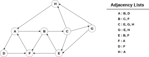
Solution:
Push H onto the stack
- STACK: H
POP the top element of the stack i.e. H, print it and push all the neighbours of H onto the stack that are is ready state.
- Print H
- STACK: A
Pop the top element of the stack i.e. A, print it and push all the neighbours of A onto the stack that are in ready state.
- Print A
- Stack: B, D
Pop the top element of the stack i.e. D, print it and push all the neighbours of D onto the stack that are in ready state.
- Print D
- Stack: B, F
Pop the top element of the stack i.e. F, print it and push all the neighbours of F onto the stack that are in ready state.
- Print F
- Stack: B
Pop the top of the stack i.e. B and push all the neighbours
- Print B
- Stack: C
Pop the top of the stack i.e. C and push all the neighbours.
- Print C
- Stack: E, G
Pop the top of the stack i.e. G and push all its neighbours.
- Print G
- Stack: E
Pop the top of the stack i.e. E and push all its neighbours.
- Print E
- Stack:
Hence, the stack now becomes empty and all the nodes of the graph have been traversed.
The printing sequence of the graph will be:
- H → A → D → F → B → C → G → E
Analysis of DFS
In the above algorithm, there is only one DFSVISIT(u) call for each vertex u in the vertex set V. Initialization complexity in DFS(G) for loop is O(V). In second for loop of DFS(G), complexity is O(V) if we leave the call of DFSVISIT(u).
Now, let us find the complexity of function DFSVISIT(u)
The complexity of for loop will be O(deg(u)+1) if we do not consider the recursive call to DFSVISIT(v). For recursive call to DFSVISIT(v), (complexity will be O(E) as
Recursive call to DFSVISIT(v) will be at most the sum of degree of adjacency for all vertex v in the vertex set V. It can be written as ∑ |Adj(v)|=O(E) vεV
The running time of DSF is (V + E).
Breadth first search
It is an uninformed search methodology which first expand and examine all nodes of graph systematically in search of the solution in the sequence and then go at the deeper level. In other words, it exhaustively searches the entire graph without considering the goal until it finds it.
From the standpoint of the algorithm, all child nodes obtained by expanding a node are added to a FIFO queue. In typical implementations, nodes that have not yet been examined for their neighbors are placed in some container (such as a queue or linked list) called "open" and then once examined are placed in the container "closed".
Steps for implementing Breadth first search
Step 1: - Initialize all the vertices by setting Flag = 1
Step 2: - Put the starting vertex A in Q and change its status to the waiting state by setting Flag = 0
Step 3: - Repeat through step 5 while Q is not NULL
Step 4: - Remove the front vertex v of Q. Process v and set the status of v to the processed status by setting Flag = -1
Step 5: - Add to the rear of Q all the neighbour of v that are in the ready state by setting Flag = 1 and change their status to the waiting state by setting flag = 0
Step 6: - Exit
Algorithm for BFS
BFS (G, s)
{
For each v in V - {s} // for loop {
color[v]=white;
d[v]= INFINITY;
p[v]=NULL;
}
color[s] = gray;
d[s]=0;
p[s]=NULL;
Q = ø; // Initialize queue is empty
Enqueue(Q, s); /* Insert start vertex s in Queue Q */
while Q is nonempty // while loop
{
u = Dequeue[Q]; /* Remove an element from Queue Q*/
for each v in Adj[u] // for loop
{ if (color[v] == white) /*if v is unvisted*/
{
Color[v] = gray; /* v is visted */
d[v] = d[u] + 1; /*Set distance of v to no. Of edges from s to u*/
p[v] = u; /*Set parent of v*/
Enqueue(Q,v); /*Insert v in Queue Q*/
}
}
color[u] = black; /*finally visted or explored vertex u*/
}
}
Breadth First Search algorithm used in
● Prim's MST algorithm.
● Dijkstra's single source shortest path algorithm.
● Testing whether graph is connected.
● Computing a cycle in graph or reporting that no such cycle exists.
Example
Consider the graph G shown in the following image, calculate the minimum path p from node A to node E. Given that each edge has a length of 1.

Solution:
Minimum Path P can be found by applying breadth first search algorithm that will begin at node A and will end at E. The algorithm uses two queues, namely QUEUE1 and QUEUE2. QUEUE1 holds all the nodes that are to be processed while QUEUE2 holds all the nodes that are processed and deleted from QUEUE1.
Let’s start examining the graph from Node A.
1. Add A to QUEUE1 and NULL to QUEUE2.
QUEUE1 = {A}
QUEUE2 = {NULL}
2. Delete the Node A from QUEUE1 and insert all its neighbours. Insert Node A into QUEUE2
QUEUE1 = {B, D}
QUEUE2 = {A}
3. Delete the node B from QUEUE1 and insert all its neighbours. Insert node B into QUEUE2.
QUEUE1 = {D, C, F}
QUEUE2 = {A, B}
4. Delete the node D from QUEUE1 and insert all its neighbours. Since F is the only neighbour of it which has been inserted, we will not insert it again. Insert node D into QUEUE2.
QUEUE1 = {C, F}
QUEUE2 = { A, B, D}
5. Delete the node C from QUEUE1 and insert all its neighbours. Add node C to QUEUE2.
QUEUE1 = {F, E, G}
QUEUE2 = {A, B, D, C}
6. Remove F from QUEUE1 and add all its neighbours. Since all of its neighbours has already been added, we will not add them again. Add node F to QUEUE2.
QUEUE1 = {E, G}
QUEUE2 = {A, B, D, C, F}
7. Remove E from QUEUE1, all of E's neighbours has already been added to QUEUE1 therefore we will not add them again. All the nodes are visited and the target node i.e. E is encountered into QUEUE2.
QUEUE1 = {G}
QUEUE2 = {A, B, D, C, F, E}
Now, backtrack from E to A, using the nodes available in QUEUE2.
The minimum path will be A → B → C → E.
Analysis of BFS
In this algorithm first for loop executes at most O(V) times.
While loop executes at most O(V) times as every vertex v in V is enqueued only once in the Queue Q. Every vertex is enqueued once and dequeued once so queuing will take at most O(V) time.
Inside while loop, there is for loop which will execute at most O(E) times as it will be at most the sum of degree of adjacency for all vertex v in the vertex set V.
Which can be written as
∑ |Adj(v)|=O(E)
vεV
Total running time of BFS is O(V + E).
Like depth first search, BFS traverse a connected component of a given graph and defines a spanning tree.
Space complexity of DFS is much lower than BFS (breadth-first search). It also lends itself much better to heuristic methods of choosing a likely-looking branch. Time complexity of both algorithms are proportional to the number of vertices plus the number of edges in the graphs they traverse.
Key takeaways
- Depth First Search is an algorithm for traversing or searching a graph.
- DFS is an uninformed search that progresses by expanding the first child node of the graph that appears and thus going deeper and deeper until a goal node is found, or until it hits a node that has no children.
- BFS is an uninformed search methodology which first expand and examine all nodes of graph systematically in search of the solution in the sequence and then goes to the deeper level.
- In other words, it exhaustively searches the entire graph without considering the goal until it finds it.
Difference between DFS and BFS
| BFS
| DFS |
Full form | BFS stands for Breadth First Search. | DFS stands for Depth First Search. |
Technique | It a vertex-based technique to find the shortest path in a graph. | It is an edge-based technique because the vertices along the edge are explored first from the starting to the end node. |
Definition | BFS is a traversal technique in which all the nodes of the same level are explored first, and then we move to the next level. | DFS is also a traversal technique in which traversal is started from the root node and explore the nodes as far as possible until we reach the node that has no unvisited adjacent nodes. |
Data Structure | Queue data structure is used for the BFS traversal. | Stack data structure is used for the BFS traversal. |
Backtracking | BFS does not use the backtracking concept. | DFS uses backtracking to traverse all the unvisited nodes. |
Number of edges | BFS finds the shortest path having a minimum number of edges to traverse from the source to the destination vertex. | In DFS, a greater number of edges are required to traverse from the source vertex to the destination vertex. |
Optimality | BFS traversal is optimal for those vertices which are to be searched closer to the source vertex. | DFS traversal is optimal for those graphs in which solutions are away from the source vertex. |
Speed | BFS is slower than DFS. | DFS is faster than BFS. |
Suitability for decision tree | It is not suitable for the decision tree because it requires exploring all the neighboring nodes first. | It is suitable for the decision tree. Based on the decision, it explores all the paths. When the goal is found, it stops its traversal. |
Memory efficient | It is not memory efficient as it requires more memory than DFS. | It is memory efficient as it requires less memory than BFS. |
Given an undirected graph, print all connected components line by line. For example consider the following graph.
We have discussed algorithms for finding strongly connected components in directed graphs in the following posts.
Kosaraju’s algorithm for strongly connected components.
Tarjan’s Algorithm to find Strongly Connected Components
Finding connected components for an undirected graph is an easier task. We simple need to do either BFS or DFS starting from every unvisited vertex, and we get all strongly connected components. Below are steps based on DFS.
1) Initialize all vertices as not visited.
2) Do the following for every vertex 'v'.
(a) If 'v' is not visited before, call DFSUtil(v)
(b) Print new line character
DFSUtil(v)
1) Mark 'v' as visited.
2) Print 'v'
3) Do the following for every adjacent 'u' of 'v'.
If 'u' is not visited, then recursively call DFSUtil(u)
Below is the implementation of the above algorithm.
// C++ program to print connected components in
// an undirected graph
#include <iostream>
#include <list>
Using namespace std;
// Graph class represents a undirected graph
// using adjacency list representation
Class Graph {
Int V; // No. Of vertices
// Pointer to an array containing adjacency lists
List<int>* adj;
// A function used by DFS
Void DFSUtil(int v, bool visited[]);
Public:
Graph(int V); // Constructor
~Graph();
Void addEdge(int v, int w);
Void connectedComponents();
};
// Method to print connected components in an
// undirected graph
Void Graph::connectedComponents()
{
// Mark all the vertices as not visited
Bool* visited = new bool[V];
For (int v = 0; v < V; v++)
Visited[v] = false;
For (int v = 0; v < V; v++) {
If (visited[v] == false) {
// print all reachable vertices
// from v
DFSUtil(v, visited);
Cout << "\n";
}
}
Delete[] visited;
}
Void Graph::DFSUtil(int v, bool visited[])
{
// Mark the current node as visited and print it
Visited[v] = true;
Cout << v << " ";
// Recur for all the vertices
// adjacent to this vertex
List<int>::iterator i;
For (i = adj[v].begin(); i != adj[v].end(); ++i)
If (!visited[*i])
DFSUtil(*i, visited);
}
Graph::Graph(int V)
{
This->V = V;
Adj = new list<int>[V];
}
Graph::~Graph() { delete[] adj; }
// method to add an undirected edge
Void Graph::addEdge(int v, int w)
{
Adj[v].push_back(w);
Adj[w].push_back(v);
}
// Driver code
Int main()
{
// Create a graph given in the above diagram
Graph g(5); // 5 vertices numbered from 0 to 4
g.addEdge(1, 0);
g.addEdge(2, 3);
g.addEdge(3, 4);
Cout << "Following are connected components \n";
g.connectedComponents();
Return 0;
}
Output:
0 1
2 3 4
Time complexity of the above solution is O (V + E) as it does simple DFS for a given graph.
Key takeaway
- Finding connected components for an undirected graph is an easier task.
- We simple need to do either BFS or DFS starting from every unvisited vertex, and we get all strongly connected components. Below are steps based on DFS.
1) Initialize all vertices as not visited.
2) Do the following for every vertex 'v'.
(a) If 'v' is not visited before, call DFSUtil(v)
(b) Print new line character
A spanning tree is a subset of Graph G that covers all of the vertices with the fewest number of edges feasible. As a result, a spanning tree has no cycles and cannot be disconnected.
We can deduce from this definition that every linked and undirected Graph G contains at least one spanning tree. Because a disconnected graph cannot be spanned to all of its vertices, it lacks a spanning tree.
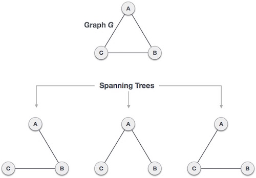
Fig: Spanning tree
From a single full graph, we discovered three spanning trees. The greatest number of spanning trees in a full undirected graph is nn-2, where n is the number of nodes. Because n is 3 in the example above, 33-2 = 3 spanning trees are conceivable.
Properties of spanning tree
We now know that a graph can contain many spanning trees. A few features of the spanning tree related to graph G are listed below.
● There can be more than one spanning tree in a linked graph G.
● The number of edges and vertices in all conceivable spanning trees of graph G is the same.
● There is no cycle in the spanning tree (loops).
● When one edge is removed from the spanning tree, the graph becomes unconnected, i.e. the spanning tree becomes minimally connected.
● When one edge is added to the spanning tree, a circuit or loop is created, indicating that the spanning tree is maximally acyclic.
Mathematical Properties of Spanning Tree
- Spanning tree has n-1 edges, where n is the number of nodes (vertices).
- From a complete graph, by removing maximum e - n + 1 edges, we can construct a spanning tree.
- A complete graph can have maximum nn-2 number of spanning trees.
Application of spanning tree
The spanning tree is used to discover the shortest path between all nodes in a graph. The use of spanning trees is common in a variety of situations.
● Civil Network Planning
● Computer Network Routing Protocol
● Cluster Analysis
Let's look at an example to help us comprehend. Consider the city network as a large graph, and the current objective is to deploy telephone lines in such a way that we can link to all city nodes with the bare minimum of lines. The spanning tree enters the scene at this point.
Key takeaway
- A spanning tree is a subset of Graph G that covers all of the vertices with the fewest amount of edges feasible.
- As a result, a spanning tree has no cycles and cannot be disconnected.
Single source shortest path problem
Introduction:
In a shortest- paths problem, we are given a weighted, directed graphs G = (V, E), with weight function w: E → R mapping edges to real-valued weights. The weight of path p = (v0,v1,..... vk) is the total of the weights of its constituent edges:

We define the shortest - path weight from u to v by δ(u,v) = min (w (p): u→v), if there is a path from u to v, and δ(u,v)= ∞, otherwise.
The shortest path from vertex s to vertex t is then defined as any path p with weight w (p) = δ(s,t).
The breadth-first- search algorithm is the shortest path algorithm that works on unweighted graphs, that is, graphs in which each edge can be considered to have unit weight.
In a Single Source Shortest Paths Problem, we are given a Graph G = (V, E), we want to find the shortest path from a given source vertex s ∈ V to every vertex v ∈ V.
Variants:
There are some variants of the shortest path problem.
- Single- destination shortest - paths problem: Find the shortest path to a given destination vertex t from every vertex v. By shift the direction of each edge in the graph, we can shorten this problem to a single - source problem.
- Single - pair shortest - path problem: Find the shortest path from u to v for given vertices u and v. If we determine the single - source problem with source vertex u, we clarify this problem also. Furthermore, no algorithms for this problem are known that run asymptotically faster than the best single - source algorithms in the worst case.
- All - pairs shortest - paths problem: Find the shortest path from u to v for every pair of vertices u and v. Running a single - source algorithm once from each vertex can clarify this problem; but it can generally be solved faster, and its structure is of interest in the own right.
Shortest Path: Existence:
If some path from s to v contains a negative cost cycle then, there does not exist the shortest path. Otherwise, there exists a shortest s - v that is simple.

Fig - Shortest Path: Existence
The single source shortest path algorithm (for arbitrary weight positive or negative) is also known Bellman-Ford algorithm is used to find minimum distance from source vertex to any other vertex. The main difference between this algorithm with Dijkstra’s algorithm is, in Dijkstra’s algorithm we cannot handle the negative weight, but here we can handle it easily.

Fig - The single source shortest path algorithm
Bellman-Ford algorithm finds the distance in bottom up manner. At first it finds those distances which have only one edge in the path. After that increase the path length to find all possible solutions.
Input − The cost matrix of the graph:
0 6 ∞ 7 ∞
∞ 0 5 8 -4
∞ -2 0 ∞ ∞
∞ ∞ -3 0 9
2 ∞ 7 ∞ 0
Output− Source Vertex: 2
Vert: 0 1 2 3 4
Dist: -4 -2 0 3 -6
Pred: 4 2 -1 0 1
The graph has no negative edge cycle
Algorithm
BellmanFord(dist, pred, source)
Input− Distance list, predecessor list and the source vertex.
Output− True, when a negative cycle is found.
Begin
ICount := 1
MaxEdge := n * (n - 1) / 2 //n is number of vertices
For all vertices v of the graph, do
Dist[v] := ∞
Pred[v] := ϕ
Done
Dist[source] := 0
ECount := number of edges present in the graph
Create edge list named edgeList
While iCount < n, do
For i := 0 to eCount, do
If dist[edgeList[i].v] > dist[edgeList[i].u] + (cost[u,v] for edge i)
Dist[edgeList[i].v] > dist[edgeList[i].u] + (cost[u,v] for edge i)
Pred[edgeList[i].v] := edgeList[i].u
Done
Done
ICount := iCount + 1
For all vertices i in the graph, do
If dist[edgeList[i].v] > dist[edgeList[i].u] + (cost[u,v] for edge i), then
Return true
Done
Return false
End
Example(C++)
#include<iostream>
#include<iomanip>
#define V 5
#define INF 999
Using namespace std;
//Cost matrix of the graph (directed) vertex 5
Int costMat[V][V] = {
{0, 6, INF, 7, INF},
{INF, 0, 5, 8, -4},
{INF, -2, 0, INF, INF},
{INF, INF, -3, 0, 9},
{2, INF, 7, INF, 0}
};
Typedef struct{
Int u, v, cost;
}edge;
Int isDiagraph(){
//check the graph is directed graph or not
Int i, j;
For(i = 0; i<V; i++){
For(j = 0; j<V; j++){
If(costMat[i][j] != costMat[j][i]){
Return 1;//graph is directed
}
}
}
Return 0;//graph is undirected
}
Int makeEdgeList(edge *eList){
//create edgelist from the edges of graph
Int count = -1;
If(isDiagraph()){
For(int i = 0; i<V; i++){
For(int j = 0; j<V; j++){
If(costMat[i][j] != 0 && costMat[i][j] != INF){
Count++;//edge find when graph is directed
EList[count].u = i; eList[count].v = j;
EList[count].cost = costMat[i][j];
}
}
}
}else{
For(int i = 0; i<V; i++){
For(int j = 0; j<i; j++){
If(costMat[i][j] != INF){
Count++;//edge find when graph is undirected
EList[count].u = i; eList[count].v = j;
EList[count].cost = costMat[i][j];
}
}
}
}
Return count+1;
}
Int bellmanFord(int *dist, int *pred,int src){
Int icount = 1, ecount, max = V*(V-1)/2;
Edge edgeList[max];
For(int i = 0; i<V; i++){
Dist[i] = INF;//initialize with infinity
Pred[i] = -1;//no predecessor found.
}
Dist[src] = 0;//for starting vertex, distance is 0
Ecount = makeEdgeList(edgeList); //edgeList formation
While(icount < V){ //number of iteration is (Vertex - 1)
For(int i = 0; i<ecount; i++){
If(dist[edgeList[i].v] > dist[edgeList[i].u] + costMat[edgeList[i].u][edgeList[i].v]){
//relax edge and set predecessor
Dist[edgeList[i].v] = dist[edgeList[i].u] + costMat[edgeList[i].u][edgeList[i].v];
Pred[edgeList[i].v] = edgeList[i].u;
}
}
Icount++;
}
//test for negative cycle
For(int i = 0; i<ecount; i++){
If(dist[edgeList[i].v] > dist[edgeList[i].u] + costMat[edgeList[i].u][edgeList[i].v]){
Return 1;//indicates the graph has negative cycle
}
}
Return 0;//no negative cycle
}
Void display(int *dist, int *pred){
Cout << "Vert: ";
For(int i = 0; i<V; i++)
Cout <<setw(3) << i << " ";
Cout << endl;
Cout << "Dist: ";
For(int i = 0; i<V; i++)
Cout <<setw(3) << dist[i] << " ";
Cout << endl;
Cout << "Pred: ";
For(int i = 0; i<V; i++)
Cout <<setw(3) << pred[i] << " ";
Cout << endl;
}
Int main(){
Int dist[V], pred[V], source, report;
Source = 2;
Report = bellmanFord(dist, pred, source);
Cout << "Source Vertex: " << source<<endl;
Display(dist, pred);
If(report)
Cout << "The graph has a negative edge cycle" << endl;
Else
Cout << "The graph has no negative edge cycle" << endl;
}
Output
Source Vertex: 2
Vert: 0 1 2 3 4
Dist: -4 -2 0 3 -6
Pred: 4 2 -1 0 1
The graph has no negative edge cycle
Key takeaway
In a shortest- paths problem, we are given a weighted, directed graphs G = (V, E), with weight function w: E → R mapping edges to real-valued weights. The weight of path p = (v0,v1,..... vk) is the total of the weights of its constituent edges:

We define the shortest - path weight from u to v by δ(u,v) = min (w (p): u→v), if there is a path from u to v, and δ(u,v)= ∞, otherwise.
The shortest path from vertex s to vertex t is then defined as any path p with weight w (p) = δ(s,t).
The breadth-first- search algorithm is the shortest path algorithm that works on unweighted graphs, that is, graphs in which each edge can be considered to have unit weight.
In a Single Source Shortest Paths Problem, we are given a Graph G = (V, E), we want to find the shortest path from a given source vertex s ∈ V to every vertex v ∈ V.
Floydd’s Algorithm for All-Pairs Shortest Paths Problem
Let the vertices of G be V = {1, 2........n} and consider a subset {1, 2........k} of vertices for some k. For any pair of vertices i, j ∈ V, considered all paths from i to j whose intermediate vertices are all drawn from {1, 2.......k}, and let p be a minimum weight path from amongst them. The Floyd-Warshall algorithm exploits a link between path p and shortest paths from i to j with all intermediate vertices in the set {1, 2.......k-1}. The link depends on whether or not k is an intermediate vertex of path p.
If k is not an intermediate vertex of path p, then all intermediate vertices of path p are in the set {1, 2........k-1}. Thus, the shortest path from vertex i to vertex j with all intermediate vertices in the set {1, 2.......k-1} is also the shortest path i to j with all intermediate vertices in the set {1, 2.......k}.
If k is an intermediate vertex of path p, then we break p down into i → k → j.
Let dij(k) be the weight of the shortest path from vertex i to vertex j with all intermediate vertices in the set {1, 2.......k}.
A recursive definition is given by
dij(k) = { wij if k = 0 min(dijk-1 , dikk-1 + dkjk-1) if k ≥ 1}
FLOYD - WARSHALL (W)
1. n ← rows [W].
2. D0← W
3. For k ← 1 to n
4. Do for i ← 1 to n
5. Do for j ← 1 to n
6. Do dij(k)← min (dij(k-1),dik(k-1)+dkj(k-1) )
7. Return D(n)
The strategy adopted by the Floyd-Warshall algorithm is Dynamic Programming. The running time of the Floyd-Warshall algorithm is determined by the triply nested for loops of lines 3-6. Each execution of line 6 takes O (1) time. The algorithm thus runs in time θ(n3 ).
Example: Apply Floyd-Warshall algorithm for constructing the shortest path. Show that matrices D(k) and π(k) computed by the Floyd-Warshall algorithm for the graph.
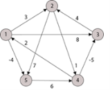
Solution:
dij(k) = min (dij(k-1), dij(k-1) + dkj(k - 1))

Step (i) When k = 0
| 3 | 8 | ∞ | -4 |
| 1 | 1 | Nil | 1 |
∞ | 0 | ∞ | 1 | 7 | Nil | Nil | Nil | 2 | 2 |
∞ | 4 | 0 | -5 | ∞ | Nil | 3 | Nil | 3 | Nil |
2 | ∞ | ∞ | 0 | ∞ | 4 | Nil | Nil | Nil | Nil |
∞ | ∞ | ∞ | 6 | 0 | Nil | Nil | Nil | 5 | Nil |
Step (ii) When k =1


| 3 | 8 | ∞ | -4 |
| 1 | 1 | Nil | 1 |
∞ | 0 | ∞ | 1 | 7 | Nil | Nil | Nil | 2 | 2 |
∞ | 4 | 0 | -5 | ∞ | Nil | 3 | Nil | 3 | Nil |
2 | 5 | 10 | 0 | -2 | 4 | 1 | 1 | Nil | 1 |
∞ | ∞ | ∞ | 6 | 0 | Nil | Nil | Nil | 5 | Nil |
Step (iii) When k = 2


Step (iv) When k = 3


| 0 | 3 | 8 | -4 |
| 1 | 1 | 3 | 1 |
∞ | 0 | ∞ | 1 | 7 | Nil | Nil | Nil | 2 | 2 |
∞ | 4 | 0 | -5 | 11 | Nil | 3 | Nil | 3 | 2 |
2 | 5 | 10 | 0 | -2 | 4 | 1 | 1 | Nil | 1 |
∞ | ∞ | ∞ | 6 | 0 | Nil | Nil | Nil | 5 | Nil |
Step (v) When k = 4


| 3 | 8 | 3 | -4 |
| 1 | 1 | 3 | 1 |
3 | 0 | 11 | 1 | -1 | 4 | Nil | 4 | 2 | 2 |
-3 | 0 | 0 | -5 | -7 | 4 | 4 | NIL | 3 | 4 |
2 | 5 | 10 | 0 | -2 | 4 | 1 | 1 | NIL | 1 |
8 | 11 | 16 | 6 | 0 | 4 | 4 | 4 | 5 | NIL |
Step (vi) When k = 5


| 3 | 8 | 3 | -4 |
| 1 | 1 | 5 | 1 |
3 | 0 | 11 | 1 | -1 | 4 | Nil | 4 | 2 | 4 |
-3 | 0 | 0 | -5 | -7 | 4 | 4 | Nil | 3 | 4 |
2 | 5 | 10 | 0 | -2 | 4 | 1 | 1 | NIL | 1 |
8 | 11 | 16 | 6 | 0 | 4 | 4 | 4 | 5 | NIL |
TRANSITIVE- CLOSURE (G)
1. n ← |V[G]|
2. For i ← 1 to n
3. Do for j ← 1 to n
4. Do if i = j or (i, j) ∈ E [G]
5. The ← 1
6. Else ← 0
7. For k ← 1 to n
8. Do for i ← 1 to n
9. Do for j ← 1 to n
10. Dod ij(k)←
11. Return T(n).
Key takeaway
The Floyd Warshall Algorithm is for solving the All Pairs Shortest Path problem.
The problem is to find shortest distances between every pair of vertices in a given edge weighted directed Graph.
The topological sorting for a directed acyclic graph is the linear ordering of vertices. For every edge U-V of a directed graph, the vertex u will come before vertex v in the ordering.
As we know that the source vertex will come after the destination vertex, so we need to use a stack to store previous elements. After completing all nodes, we can simply display them from the stack.
Input and Output
Input:
0 0 0 0 0 0
0 0 0 0 0 0
0 0 0 1 0 0
0 1 0 0 0 0
1 1 0 0 0 0
1 0 1 0 0 0
Output:
Nodes after topological sorted order: 5 4 2 3 1 0
Algorithm
TopoSort(u, visited, stack)
Input − The start vertex u, An array to keep track of which node is visited or not. A stack to store nodes.
Output − Sorting the vertices in topological sequence in the stack.
Begin
Mark u as visited
For all vertices v which is adjacent with u, do
If v is not visited, then
TopoSort(c, visited, stack)
Done
Push u into a stack
End
Perform Topological Sorting(Graph)
Input − The given directed acyclic graph.
Output − Sequence of nodes.
Begin
Initially mark all nodes as unvisited
For all nodes v of the graph, do
If v is not visited, then
TopoSort(i, visited, stack)
Done
Pop and print all elements from the stack
End.
Example
#include<iostream>
#include<stack>
#define NODE 6
Using namespace std;
Int graph[NODE][NODE] = {
{0, 0, 0, 0, 0, 0},
{0, 0, 0, 0, 0, 0},
{0, 0, 0, 1, 0, 0},
{0, 1, 0, 0, 0, 0},
{1, 1, 0, 0, 0, 0},
{1, 0, 1, 0, 0, 0}
};
Void topoSort(int u, bool visited[], stack<int>&stk) {
Visited[u] = true; //set as the node v is visited
For(int v = 0; v<NODE; v++) {
If(graph[u][v]) { //for allvertices v adjacent to u
If(!visited[v])
TopoSort(v, visited, stk);
}
}
Stk.push(u); //push starting vertex into the stack
}
Void performTopologicalSort() {
Stack<int> stk;
Bool vis[NODE];
For(int i = 0; i<NODE; i++)
Vis[i] = false; //initially all nodes are unvisited
For(int i = 0; i<NODE; i++)
If(!vis[i]) //when node is not visited
TopoSort(i, vis, stk);
While(!stk.empty()) {
Cout <<stk.top() << " ";
Stk.pop();
}
}
Main() {
Cout << "Nodes after topological sorted order: ";
PerformTopologicalSort();
}
Output
Nodes after topological sorted order: 5 4 2 3 1 0
We must use the Backtracking technique to identify the Hamiltonian Circuit given a graph G = (V, E). We begin our search at any random vertex, such as 'a.' The root of our implicit tree is this vertex 'a.' The first intermediate vertex of the Hamiltonian Cycle to be constructed is the first element of our partial solution. By alphabetical order, the next nearby vertex is chosen.
A dead end is reached when any arbitrary vertices forms a cycle with any vertex other than vertex 'a' at any point. In this situation, we backtrack one step and restart the search by selecting a new vertex and backtracking the partial element; the answer must be removed. If a Hamiltonian Cycle is found, the backtracking search is successful.
Example - Consider the graph G = (V, E) in fig. We must use the Backtracking method to find a Hamiltonian circuit.
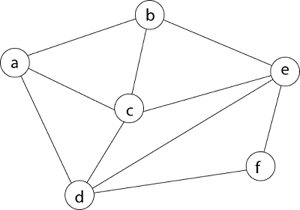
To begin, we'll start with vertex 'a,' which will serve as the root of our implicit tree.

Following that, we select the vertex 'b' adjacent to 'a' because it is the first in lexicographical order (b, c, d).

Then, next to 'b,' we select 'c.'

Next, we choose the letter 'd,' which is adjacent to the letter 'c.'

Then we select the letter 'e,' which is adjacent to the letter 'd.'
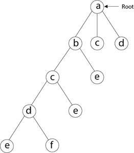
Then, adjacent to 'e,' we select vertex 'f.' D and e are the vertex next to 'f,' but they've already been there. As a result, we reach a dead end and go back a step to delete the vertex 'f' from the partial solution.
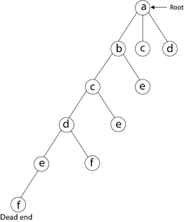
The vertices adjacent to 'e' is b, c, d, and f, from which vertex 'f' has already been verified, and b, c, and d have previously been visited, according to backtracking. As a result, we go back one step. The vertex adjacent to d is now e, f, from which e has already been checked, and the vertex adjacent to 'f' is now d and e. We get a dead state if we revisit the 'e' vertex. As a result, we go back one step.
References:
1. Aaron M. Tenenbaum, Yedidyah Langsam and Moshe J. Augenstein, “Data Structures Using C and C++”, PHI Learning Private Limited, Delhi India
2. Horowitz and Sahani, “Fundamentals of Data Structures”, Galgotia Publications Pvt Ltd Delhi India.
3. Lipschutz, “Data Structures” Schaum’s Outline Series, Tata McGraw-hill Education (India) Pvt. Ltd.Thareja, “Data Structure Using C” Oxford Higher Education.
4. AK Sharma, “Data Structure Using C”, Pearson Education India.