Unit - 3
Physical and logical hierarchy
Indexing in DBMS
● Indexing is used to optimize the performance of a database by minimizing the number of disk accesses required when a query is processed.
● The index is a type of data structure. It is used to locate and access the data in a database table quickly.
Index structure:
Indexes can be created using some database columns.

Fig 6: Structure of Index
● The first column of the database is the search key that contains a copy of the primary key or candidate key of the table. The values of the primary key are stored in sorted order so that the corresponding data can be accessed easily.
● The second column of the database is the data reference. It contains a set of pointers holding the address of the disk block where the value of the particular key can be found.
Indexing Methods
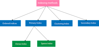
Fig 1: Indexing Methods
Ordered indices
The indices are usually sorted to make searching faster. The indices which are sorted are known as ordered indices.
Example: Suppose we have an employee table with thousands of records and each of which is 10 bytes long. If their IDs start with 1, 2, 3....and so on and we have to search student with ID-543.
● In the case of a database with no index, we have to search the disk block from starting till it reaches 543. The DBMS will read the record after reading 543*10=5430 bytes.
● In the case of an index, we will search using indexes and the DBMS will read the record after reading 542*2= 1084 bytes which are very less compared to the previous case.
Primary Index
● If the index is created on the basis of the primary key of the table, then it is known as primary indexing. These primary keys are unique to each record and contain 1:1 relation between the records.
● As primary keys are stored in sorted order, the performance of the searching operation is quite efficient.
● The primary index can be classified into two types: Dense index and Sparse index.
Dense index
● The dense index contains an index record for every search key value in the data file. It makes searching faster.
● In this, the number of records in the index table is same as the number of records in the main table.
● It needs more space to store index record itself. The index records have the search key and a pointer to the actual record on the disk.

Fig 2: Dense Index
Sparse index
● In the data file, index record appears only for a few items. Each item points to a block.
● In this, instead of pointing to each record in the main table, the index points to the records in the main table in a gap.

Fig 3: Sparse Index
Clustering Index
● A clustered index can be defined as an ordered data file. Sometimes the index is created on non-primary key columns which may not be unique for each record.
● In this case, to identify the record faster, we will group two or more columns to get the unique value and create index out of them. This method is called a clustering index.
● The records which have similar characteristics are grouped, and indexes are created for these group.
Example: suppose a company contains several employees in each department. Suppose we use a clustering index, where all employees which belong to the same Dept_ID are considered within a single cluster, and index pointers point to the cluster as a whole. Here Dept_Id is a non-unique key.
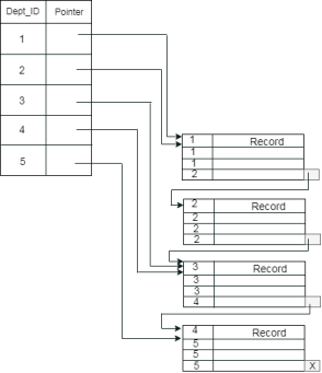
The previous schema is little confusing because one disk block is shared by records which belong to the different cluster. If we use separate disk block for separate clusters, then it is called better technique.
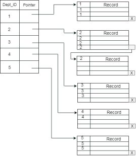
Secondary Index
In the sparse indexing, as the size of the table grows, the size of mapping also grows. These mappings are usually kept in the primary memory so that address fetch should be faster. Then the secondary memory searches the actual data based on the address got from mapping. If the mapping size grows then fetching the address itself becomes slower. In this case, the sparse index will not be efficient. To overcome this problem, secondary indexing is introduced.
In secondary indexing, to reduce the size of mapping, another level of indexing is introduced. In this method, the huge range for the columns is selected initially so that the mapping size of the first level becomes small. Then each range is further divided into smaller ranges. The mapping of the first level is stored in the primary memory, so that address fetch is faster. The mapping of the second level and actual data are stored in the secondary memory (hard disk).
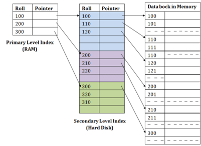
Fig 10: Secondary Index
For example:
● If you want to find the record of roll 111 in the diagram, then it will search the highest entry which is smaller than or equal to 111 in the first level index. It will get 100 at this level.
● Then in the second index level, again it does max (111) <= 111 and gets 110. Now using the address 110, it goes to the data block and starts searching each record till it gets 111.
● This is how a search is performed in this method. Inserting, updating or deleting is also done in the same manner.
Key takeaway
● Indexing is used to optimize the performance of a database by minimizing the number of disk accesses required when a query is processed.
● The index is a type of data structure. It is used to locate and access the data in a database table quickly.
A self-balancing search tree is a B-Tree. It is presumed that everything is in the primary memory of most other self-balancing search trees (such as AVL and Red-Black Trees). We have to think of the vast amount of data that can not fit into the main memory to understand the use of B-Trees. When the number of keys is high, data in the form of blocks is read from the disc. Compared to the principal memory access time, disc access time is very high.
The key idea of using B-Trees is to decrease the amount of access to the disc. Most tree operations (search, insert, delete, max, min, ..etc) include access to the O(h) disc where the height of the tree is h. The B-tree is a tree with fat.
By placing the maximum possible keys into a B-Tree node, the height of the B-Trees is kept low. The B-Tree node size is usually held equal to the size of the disc block. Since the B-tree height is poor, total disc access is drastically reduced compared to balanced binary search trees such as AVL Tree, Red-Black Tree, etc. for most operations.
Time Complexity of B - tree
S.no. | Algorithm | Time complexity |
1 | Search | O ( log n) |
2 | Insert | O ( log n) |
3 | Delete | O ( log n) |
n is the total no. Of elements
All the properties of an M-way tree are found in the B tree of order m. Furthermore, it includes the properties below.
● In a B-Tree, each node contains a maximum of m children.
● With the exception of the root node and the leaf node, each node in the B-Tree contains at least m/2 kids.
● There must be at least 2 nodes for the root nodes.
● It is important to have all leaf nodes at the same level.
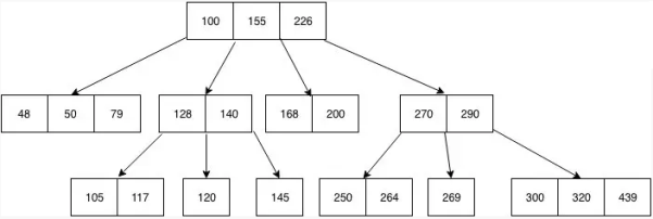
Fig 11: Example of B - tree
The minimum height of the B-Tree that can exist with n node numbers and m is the maximum number that a node can have of children is:
hmin = [logm (n+1)] - 1
The maximum height of the B-Tree that can exist with n node numbers and d is the minimum number of children that can have a non-root node:

And

Traversal in B - tree
Traversal is also similar to Binary Tree's Inorder Traversal. We start with the leftmost child, print the leftmost child recursively, then repeat the same method for the remaining children and keys. In the end, print the rightmost child recursively.
Search operation in B - tree
A search in the Binary Search Tree is equivalent to a search. Let the search key be k. We begin from the root and traverse down recursively. For any non-leaf node visited, we simply return the node if the node has the key. Otherwise, we return to the appropriate child of the node (the child who is just before the first big key). If a leaf node is reached, and k is not contained in the leaf node, then NULL is returned.
Example: Searching 120 in the given B-Tree.

Fig 12: Example for searching operation
Solution:


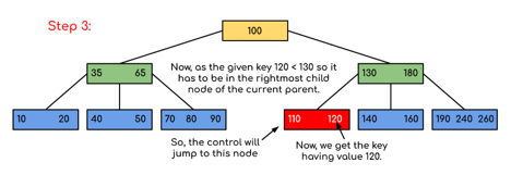
Fig 13: Steps of searching
Key takeaway:
● A self-balancing search tree is a B-Tree.
● The key idea of using B-Trees is to decrease the amount of access to the disc.
● The B-Tree node size is usually held equal to the size of the disc block.
Functional Dependency (FD) is a constraint in a database management system that specifies the relationship of one attribute to another attribute (DBMS). Functional Dependency helps to maintain the database's data quality. Finding the difference between good and poor database design plays a critical role.
The arrow "→" signifies a functional dependence. X→ Y is defined by the functional dependence of X on Y.
Rules of functional dependencies
The three most important rules for Database Functional Dependence are below:
● Reflexive law: X holds a value of Y if X is a set of attributes and Y is a subset of X.
● Augmentation rule: If x -> y holds, and c is set as an attribute, then ac -> bc holds as well. That is to add attributes that do not modify the fundamental dependencies.
● Transitivity law: If x -> y holds and y -> z holds, this rule is very similar to the transitive rule in algebra, then x -> z also holds. X -> y is referred to as functionally evaluating y.
Types of functional dependency
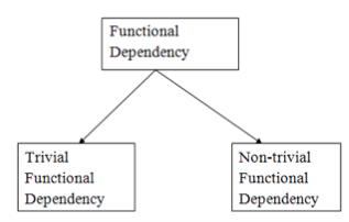
Fig 14: Types of functional dependency
1. Trivial functional dependency
● A → B has trivial functional dependency if B is a subset of A.
● The following dependencies are also trivial like: A → A, B → B
Example
Consider a table with two columns Employee_Id and Employee_Name.
{Employee_id, Employee_Name} → Employee_Id is a trivial functional dependency as
Employee_Id is a subset of {Employee_Id, Employee_Name}.
Also, Employee_Id → Employee_Id and Employee_Name → Employee_Name are trivial dependencies too.
2. Non - trivial functional dependencies
● A → B has a non-trivial functional dependency if B is not a subset of A.
● When A intersection B is NULL, then A → B is called as complete non-trivial.
Example:
ID → Name,
Name → DOB
Key takeaway:
- The arrow "→" signifies a functional dependence.
- Functional Dependency helps to maintain the database's data quality.
Normalization is often executed as a series of different forms. Each normal form has its own properties. As normalization proceeds, the relations become progressively more restricted in format, and also less vulnerable to update anomalies. For the relational data model, it is important to bring the relation only in first normal form (1NF) that is critical in creating relations. All the remaining forms are optional.
A relation R is said to be normalized if it does not create any anomaly for three basic operations: insert, delete and update.
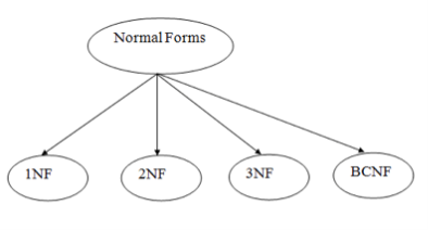
Fig 15: Types of normal forms
1NF
If a relation has an atomic value, it is in 1NF.
2NF
If a relation is in 1NF and all non-key attributes are fully functioning and dependent on the primary key, it is in 2NF.
3NF
If a relation is in 2NF and there is no transition dependency, it is in 3NF.
4NF
If a relation is in Boyce Codd normal form and has no multivalued dependencies, it is in 4NF.
5NF
If a relation is in 4NF and does not contain any join dependencies, it is in 5NF, and joining should be lossless.
Objectives of Normalization
● It is used to delete redundant information and anomalies in the database from the relational table.
● Normalization improves by analyzing new data types used in the table to reduce consistency and complexity.
● Dividing the broad database table into smaller tables and connecting them using a relationship is helpful.
● This avoids duplicating data into a table or not repeating classes.
● It decreases the probability of anomalies in a database occurring.
Key takeaway:
- Normalization is a method of arranging the database data to prevent data duplication, anomaly of addition, anomaly of update & anomaly of deletion.
- Standard types are used in database tables to remove or decrease redundancies.
Data analysis is the act of analyzing, cleansing, manipulating, and modeling data in order to find usable information, draw conclusions, and aid decision-making.
Types of Data Analysis
There are a variety of data analysis approaches that cover a wide range of areas, including business, science, and social science, and go by a variety of names. The most common data analysis methods are:
● Data Mining
● Business Intelligence
● Statistical Analysis
● Predictive Analytics
● Text Analytics
Data Mining
Data mining is the process of analyzing vast amounts of facts in order to discover previously unknown patterns, unexpected data, and dependencies. It's important to remember that the purpose is to extract patterns and insights from massive amounts of data, not to extract data itself.
Computer science methods at the junction of artificial intelligence, machine learning, statistics, and database systems are used in data mining analysis.
Data mining patterns can be thought of as a summary of the input data that can be used for further analysis or to help a decision support system provide more accurate prediction results.
Business Intelligence
Business intelligence techniques and tools are used to help find, develop, and create new strategic corporate possibilities by acquiring and transforming massive amounts of unstructured business data.
The purpose of business intelligence is to make it simple to comprehend massive amounts of data in order to find new opportunities. It assists in the implementation of an effective strategy based on insights that can give organizations a competitive market advantage as well as long-term stability.
Statistical Analysis
The study of data collection, analysis, interpretation, presentation, and organization is known as statistics.
There are two main statistical approaches used in data analysis:
Descriptive statistics − Data from the full population or a sample is summarized with numerical descriptors such as in descriptive statistics.
● Mean, Standard Deviation for Continuous Data
● Frequency, Percentage for Categorical Data
Inferential statistics − It makes inferences about the represented population or accounts for randomness using patterns in the sample data. These implications can be interpreted in a variety of ways.
● answering yes/no questions about the data (hypothesis testing)
● estimating numerical characteristics of the data (estimation)
● describing associations within the data (correlation)
● modeling relationships within the data (E.g. Regression analysis)
Predictive Analytics
Predictive analytics analyses current and historical data to make predictions about future or otherwise unknown events using statistical models. Predictive analytics is used in business to detect hazards and opportunities to help in decision-making.
Text Analytics
The technique of extracting high-quality information from text is known as text analytics, sometimes known as text mining or text data mining. Text mining often entails structuring the input text, identifying patterns within the structured data using techniques such as statistical pattern learning, and then evaluating and interpreting the results.
Data Analysis Process
"Procedures for analysing data, techniques for interpreting the results of such procedures, ways of planning the gathering of data to make its analysis easier, more precise, or more accurate, and all the machinery and results of (mathematical) statistics which apply to analysing data," according to statistician John Tukey in 1961.
As a result, data analysis is the process of acquiring huge amounts of unstructured data from a variety of sources and transforming it into information that can be used for a variety of purposes.
● Answering questions
● Test hypotheses
● Decision-making
● Disproving theories
References:
- Korth, Silbertz, Sudarshan,” Database Concepts”, McGraw Hill
- Date C J, “An Introduction to Database Systems”, Addision Wesley
- Elmasri, Navathe, “Fundamentals of Database Systems”, Addision Wesley
- O’Neil, Databases, Elsevier Pub.
- Https://www.tutorialspoint.com/excel_data_analysis/data_analysis_overview.htm