Unit - 6
Statistics and finite differences
Fitting of straight line y = a + bx, Parabola y = a + bx + c and Exponential curves by method of least squares
Method of Least Squares
Let  (1)
(1)
Be the straight line to be fitted to the given data points

Let  be the theoretical value for
Then, 


For S to be minimum


On simplification equation (2) and (3) becomes


The equation (3) and (4) are known as Normal equations.
On solving ( 3) and (4) we get the values of a and b
(b)To fit the parabola

The normal equations are 


On solving three normal equations we get the values of a,b and c.
Example. Find the best values of a and b so that y = a + bx fits the data given in the table
x | 0 | 1 | 2 | 3 | 4 |
y | 1.0 | 2.9 | 4.8 | 6.7 | 8.6 |
Solution.
y = a + bx
x | y | Xy |  |
0 | 1.0 | 0 | 0 |
1 | 2.9 | 2.0 | 1 |
2 | 4.8 | 9.6 | 4 |
3 | 6.7 | 20.1 | 9 |
4 | 8.6 | 13.4 | 16 |
 |  |  |  |
Normal equations,  y= na+ b
 x (2)
x (2)

On putting the values of 


On solving (4) and (5) we get,

On substituting the values of a and b in (1) we get

Example. By the method of least squares, find the straight line that best fits the following data:
x | 1 | 2 | 3 | 4 | 5 |
y | 14 | 27 | 40 | 55 | 68 |
Solution. Let the equation of the straight line best fit be y = a + bx. (1)
x | y | x y |  |
1 | 14 | 14 | 1 |
2 | 27 | 54 | 4 |
3 | 40 | 120 | 9 |
4 | 55 | 220 | 16 |
5 | 68 | 340 | 25 |
 |  |  |  |
Normal equations are 

On putting the values of  x,
x,  y,
y,  xy and
  in (2) and (3) we have


On solving equations (4) and (5) we get

On substituting the values of (a) and (b) in (1) we get,

Example: Find the straight line that best fits of the following data by using method of least square.
X | 1 | 2 | 3 | 4 | 5 |
y | 14 | 27 | 40 | 55 | 68 |
Sol.
Suppose the straight line
y = a + bx…….. (1)
Fits the best-
Then-
x | y | Xy |  |
1 | 14 | 14 | 1 |
2 | 27 | 54 | 4 |
3 | 40 | 120 | 9 |
4 | 55 | 220 | 16 |
5 | 68 | 340 | 25 |
Sum = 15 | 204 | 748 | 55 |
Normal equations are-


Put the values from the table, we get two normal equations-


On solving the above equations, we get-

So that the best fit line will be- (on putting the values of a and b in equation (1))

Example. Find the least squares approximation of second degree for the discrete data
x | 2 | -1 | 0 | 1 | 2 |
y | 15 | 1 | 1 | 3 | 19 |
Solution. Let the equation of second degree polynomial be 
x | y | Xy |  |  |  |  |
-2 | 15 | -30 | 4 | 60 | -8 | 16 |
-1 | 1 | -1 | 1 | 1 | -1 | 1 |
0 | 1 | 0 | 0 | 0 | 0 | 0 |
1 | 3 | 3 | 1 | 3 | 1 | 1 |
2 | 19 | 38 | 4 | 76 | 8 | 16 |
 |  |  |  |  |  |  |
Normal equations are 


On putting the values of  x,
x,  y,
y, xy,
xy,
 have
have


On solving (5),(6),(7), we get, 
The required polynomial of second degree is

Second degree parabolas and more general curves
Change of scale
If the data is of equal interval in large numbers then we change the scale as 
Example. Fit a second degree parabola to the following data by least square method:
x | 1929 | 1930 | 1931 | 1932 | 1933 | 1934 | 1935 | 1936 | 1937 |
y | 352 | 356 | 357 | 358 | 360 | 361 | 365 | 360 | 359 |
Solution. Taking 
Taking 

The equation  is transformed to
x |  | y |  | Uv |  |  |  |  |
1929 | -4 | 352 | -5 | 20 | 16 | -80 | -64 | 256 |
1930 | -3 | 360 | -1 | 3 | 9 | -9 | -27 | 81 |
1931 | -2 | 357 | 0 | 0 | 4 | 0 | -8 | 16 |
1932 | -1 | 358 | 1 | -1 | 1 | 1 | -1 | 1 |
1933 | 0 | 360 | 3 | 0 | 0 | 0 | 0 | 0 |
1934 | 1 | 361 | 4 | 4 | 1 | 4 | 1 | 1 |
1935 | 2 | 361 | 4 | 8 | 4 | 16 | 8 | 16 |
1936 | 3 | 360 | 3 | 9 | 9 | 27 | 27 | 81 |
1937 | 4 | 350 | 2 | 8 | 16 | 32 | 64 | 256 |
Total |  |
|  |  |  |  |  |  |
Normal equations are


On solving these equations we get 


Example. Fit a second degree parabola to the following data.
x=1.0 | 1.5 | 2.0 | 2.5 | 3.0 | 3.5 | 4.0 |
y=1.1 | 1.3 | 1.6 | 2.0 | 2.7 | 3.4 | 4.1 |
Solution. We shift the origin to (2.5, 0) antique 0.5 as the new unit. This amounts to changing the variable x to X, by the relation X = 2x – 5.
Let the parabola of fit be y = a + bX The values of
  X etc. Are calculated as below:
x | X | y | Xy |  |  |  |  |
1.0 | -3 | 1.1 | -3.3 | 9 | 9.9 | -27 | 81 |
1.5 | -2 | 1.3 | -2.6 | 4 | 5.2 | -5 | 16 |
2.0 | -1 | 1.6 | -1.6 | 1 | 1.6 | -1 | 1 |
2.5 | 0 | 2.0 | 0.0 | 0 | 0.0 | 0 | 0 |
3.0 | 1 | 2.7 | 2.7 | 1 | 2.7 | 1 | 1 |
3.5 | 2 | 3.4 | 6.8 | 4 | 13.6 | 8 | 16 |
4.0 | 3 | 4.1 | 12.3 | 9 | 36.9 | 27 | 81 |
Total | 0 | 16.2 | 14.3 | 28 | 69.9 | 0 | 196 |
The normal equations are
7a + 28c =16.2; 28b =14.3; 28a +196c=69.9
Solving these as simultaneous equations we get


Replacing X bye 2x – 5 in the above equation we get

Which simplifies to y = This is the required parabola of the best fit
Example: Find the least squares approximation of second degree for the discrete data
x | 2 | -1 | 0 | 1 | 2 |
y | 15 | 1 | 1 | 3 | 19 |
Solution. Let the equation of second degree polynomial be 
x | y | Xy |  |  |  |  |
-2 | 15 | -30 | 4 | 60 | -8 | 16 |
-1 | 1 | -1 | 1 | 1 | -1 | 1 |
0 | 1 | 0 | 0 | 0 | 0 | 0 |
1 | 3 | 3 | 1 | 3 | 1 | 1 |
2 | 19 | 38 | 4 | 76 | 8 | 16 |
 |  |  |  |  |  |  |
Normal equations are 


On putting the values of  x,
x,  y,
y, xy,
xy,
 have
have


On solving (5),(6),(7), we get, 
The required polynomial of second degree is

Example: Fit a second degree parabola to the following data.
X = 1.0 | 1.5 | 2.0 | 2.5 | 3.0 | 3.5 | 4.0 |
Y = 1.1 | 1.3 | 1.6 | 2.0 | 2.7 | 3.4 | 4.1 |
Solution
We shift the origin to (2.5, 0) antique 0.5 as the new unit. This amounts to changing the variable x to X, by the relation X = 2x – 5.
Let the parabola of fit be y = a + bX The values of
  X etc. Are calculated as below:
x | X | y | Xy |  |  |  |  |
1.0 | -3 | 1.1 | -3.3 | 9 | 9.9 | -27 | 81 |
1.5 | -2 | 1.3 | -2.6 | 4 | 5.2 | -5 | 16 |
2.0 | -1 | 1.6 | -1.6 | 1 | 1.6 | -1 | 1 |
2.5 | 0 | 2.0 | 0.0 | 0 | 0.0 | 0 | 0 |
3.0 | 1 | 2.7 | 2.7 | 1 | 2.7 | 1 | 1 |
3.5 | 2 | 3.4 | 6.8 | 4 | 13.6 | 8 | 16 |
4.0 | 3 | 4.1 | 12.3 | 9 | 36.9 | 27 | 81 |
Total | 0 | 16.2 | 14.3 | 28 | 69.9 | 0 | 196 |
The normal equations are
7a + 28c =16.2; 28b =14.3;. 28a +196c=69.9
Solving these as simultaneous equations we get


Replacing X bye 2x – 5 in the above equation we get

Which simplifies to y =
This is the required parabola of the best fit.
Example: Fit the curve  by using the method of least square.
X | 1 | 2 | 3 | 4 | 5 | 6 |
Y | 7.209 | 5.265 | 3.846 | 2.809 | 2.052 | 1.499 |
Sol.
Here-


Now put-
Then we get-

x | Y |  | XY |  |
1 | 7.209 | 1.97533 | 1.97533 | 1 |
2 | 5.265 | 1.66108 | 3.32216 | 4 |
3 | 3.846 | 1.34703 | 4.04109 | 9 |
4 | 2.809 | 1.03283 | 4.13132 | 16 |
5 | 2.052 | 0.71881 | 3.59405 | 25 |
6 | 1.499 | 0.40480 | 2.4288 | 36 |
Sum = 21 |
| 7.13988 | 19.49275 | 91 |
Normal equations are-

Putting the values form the table, we get-
7.13988 = 6c + 21b
19.49275 = 21c + 91b
On solving, we get-
b = -0.3141 and c = 2.28933
c = 
Now put these values in equations (1), we get-

Example: Estimate the chlorine residual in a swimming pool 5 hours after it has been treated with chemicals by fitting an exponential curve of the form
 of the data given below-
Hours(X) | 2 | 4 | 6 | 8 | 10 | 12 |
Chlorine residuals (Y) | 1.8 | 1.5 | 1.4 | 1.1 | 1.1 | 0.9 |
Sol.

Taking log on the curve which is non-linear,
We get-

Put


Then-

Which is the linear equation in X,
Its normal equations are-

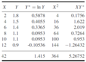
Here N = 6,


Thus the normal equations are-


On solving, we get


Or
A = 2.013 and B = 0.936
Hence the required least square exponential curve-

Prediction-
Chlorine content after 5 hours-

Correlation:
So far we have confined our attention to the analysis of observation on a single variable. There are, however, many phenomena where the changes in one variable are related to the changes in the other variable. For instance, the yield of crop varies with the amount of rainfall, the price of a commodity increases with the reduction in its supply and so on. Such a simultaneous variation, i.e., when the changes in one variable are associated or followed by change in the other, is called correlation. Such a data connecting two variables is called bivariate population.
If an increase (or decrease) in the values of one variable corresponds to an increase (or decrease) in the other, the correlation is said to be positive. If the increase (or decrease) in one corresponds to the decrease (or increase) in other, the correlation is said to be negative. If there is no relationship indicated between the variables, they are said to be independent or uncorrelated.
When two variables are related in such a way that change in the value of one variable affects the value of the other variable, then these two variables are said to be correlated and there is correlation between two variables.
Example- Height and weight of the persons of a group.
The correlation is said to be perfect correlation if two variables vary in such a way that their ratio is constant always.
Types of correlation:
According to the direction of change in variables there are two types of correlation
1. Positive Correlation
2. Negative Correlation
1. Positive Correlation:
Correlation between two variables is said to be positive if the values of the variables deviate in the same direction i.e. if the values of one variable increase (or decrease) then the values of other variable also increase (or decrease). For example:
1. Heights and weights of group of persons;
2. House hold income and expenditure;
3. Amount of rainfall and yield of crops
2. Negative Correlation:
Correlation between two variables is said to be negative if the values of variables deviate in opposite direction i.e. if the values of one variable increase (or decrease) then the values of other variable decrease (or increase). Some examples of negative correlations are correlation between
1. Volume and pressure of perfect gas;
2. Price and demand of goods;
3. Literacy and poverty in a country
Scatter diagram-
Scatter diagram is a statistical tool for determining the potentiality of correlation between dependent variable and independent variable. Scatter diagram does not tell about exact relationship between two variables but it indicates whether they are correlated or not.
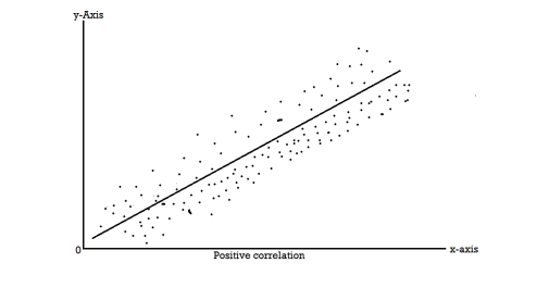
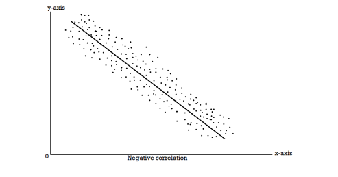
To obtain a measure of relationship between the two variables, we plot their corresponding values on the graph, taking one of the variables along the x-axis and the other along the y-axis.
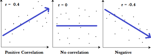
Correlation measures the nature and strength of relationship between two variables. Correlation lies between +1 to -1. A correlation of +1 indicates a perfect positive correlation between two variables. A zero correlation indicates that there is no relationship between the variables. A correlation of -1 indicates a perfect negative correlation.
Definition-
“Correlation analysis deals with the association between two or more variables.” —Simpson and Kafka
“Correlation is an analysis of the co-variation between two variables.” —A.M. Tuttle
Methods of computing coefficient of correlation
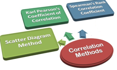
- Scatter diagram method-
It is the simplest method to study correlation between two variables. The correlations of two variables are plotted in the graph in the form of dots thereby obtaining as many points as the number of observations. The degree of correlation is ascertained by looking at the scattered points over the charts.
The more the points plotted are scattered over the chart, the lesser is the degree of correlation between the variables. The more the points plotted are closer to the line, the higher is the degree of correlation. The degree of correlation is denoted by “r”.
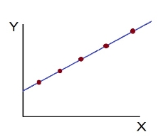
- Perfect positive correlation (r = +1) – All the points plotted on the straight line rising from left to right
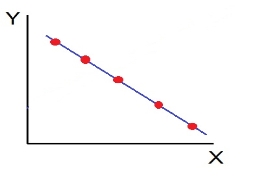
- Perfect negative correlation (r=-1) – all the points plotted on the straight line falling from left to right
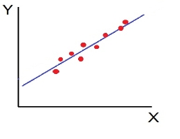
- High Degree of +Ve Corr elation (r= + High): all the points plotted close to the straight line rising from left to right
- High Degree of –Ve Correlation (r= – High) - all the points plotted close to the straight line falling from left to right.
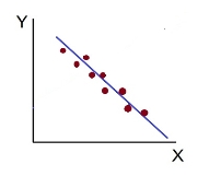
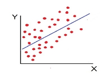
- Low degree of +Ve Correlation (r= + Low): all the points are highly scattered to the straight line rising from left to right
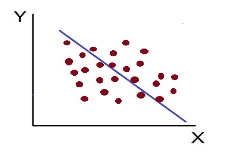
- Low Degree of –Ve Correlation (r= - Low): all the points are highly scattered to the straight line falling from left to right
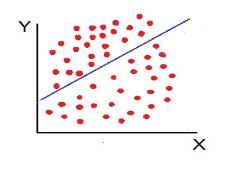
- No Correlation (r= 0) – all the points are scattered over the graph and do not show any pattern
2. Karl Pearson’s coefficient of correlation:
Coefficient of correlation measures the intensity or degree of linear relationship between two variables. It was given by British Biometrician Karl Pearson (1867-1936).
Karl Pearson’s Coefficient of Correlation is widely used mathematical method is used to calculate the degree and direction of the relationship between linear related variables. The coefficient of correlation is denoted by “r”.
If X and Y are two random variables then correlation coefficient between X and Y is denoted by r and defined as-
Karl Pearson’s coefficient of correlation-

Here-  and
and 

Note-
1. Correlation coefficient always lies between -1 and +1.
2. Correlation coefficient is independent of change of origin and scale.
3. If the two variables are independent then correlation coefficient between them is zero.
Correlation coefficient | Type of correlation |
+1 | Perfect positive correlation |
-1 | Perfect negative correlation |
0.25 | Weak positive correlation |
0.75 | Strong positive correlation |
-0.25 | Weak negative correlation |
-0.75 | Strong negative correlation |
0 | No correlation |
Example: Find the correlation coefficient between Age and weight of the following data-
Age | 30 | 44 | 45 | 43 | 34 | 44 |
Weight | 56 | 55 | 60 | 64 | 62 | 63 |
Sol.
x | Y |  |  |  |  | (   |
30 | 56 | -10 | 100 | -4 | 16 | 40 |
44 | 55 | 4 | 16 | -5 | 25 | -20 |
45 | 60 | 5 | 25 | 0 | 0 | 0 |
43 | 64 | 3 | 9 | 4 | 16 | 12 |
34 | 62 | -6 | 36 | 2 | 4 | -12 |
44 | 63 | 4 | 16 | 3 | 9 | 12 |
Sum= 240 |
360 |
0 |
202 |
0 |
70
|
32 |
Karl Pearson’s coefficient of correlation-

Here the correlation coefficient is 0.27.which is the positive correlation (weak positive correlation), this indicates that the as age increases, the weight also increase.
Short-cut method to calculate correlation coefficient-

Here,


Example: Find the correlation coefficient between the values X and Y of the dataset given below by using short-cut method-
X | 10 | 20 | 30 | 40 | 50 |
Y | 90 | 85 | 80 | 60 | 45 |
Sol.
X | Y |  |  |  |  |  |
10 | 90 | -20 | 400 | 20 | 400 | -400 |
20 | 85 | -10 | 100 | 15 | 225 | -150 |
30 | 80 | 0 | 0 | 10 | 100 | 0 |
40 | 60 | 10 | 100 | -10 | 100 | -100 |
50 | 45 | 20 | 400 | -25 | 625 | -500 |
Sum = 150 |
360 |
0 |
1000 |
10 |
1450 |
-1150 |
Short-cut method to calculate correlation coefficient-


Example
Psychological tests of intelligence and of engineering ability were applied to 10 students. Here is a record of ungrouped data showing intelligence ratio (I.R) and engineering ratio (E.R). Calculate the co-efficient of correlation.
Student | A | B | C | D | E | F | G | H | I | J |
I.R | 105 | 104 | 102 | 101 | 99 | 98 | 96 | 92 | 93 | 92 |
E.R | 101 | 103 | 100 | 98 | 96 | 104 | 92 | 94 | 97 | 94 |
Solution:
We construct the following table:
Student | Intelligence ratio   | Engineering ratio   |  |  |  |
A B C D E F G H I J | 100 6 104 5 102 3 101 2 100 1 99 0 98 -1 96 -3 93 -6 92 -7 | 101 3 103 5 100 2 98 0 95 -3 96 -2 104 6 92 -6 97 -1 94 -4 | 36 25 9 4 1 0 1 9 36 49 | 9 25 4 0 9 4 36 36 1 16 | 18 25 6 0 -3 0 -6 18 6 28 |
Total | 990 0 | 980 0 | 170 | 140 | 92 |
From this table, mean of  i.e.,
i.e.,  and mean of
  , i.e.,

Substituting these values in the formula (1), we have

Other examples:
Example-1-Compute Pearsons coefficient of correlation between advertisement cost and sales as per the data given below:
Advertisement cost | 39 | 65 | 62 | 90 | 82 | 75 | 25 | 98 | 36 | 78 |
Sales | 47 | 53 | 58 | 86 | 62 | 68 | 60 | 91 | 51 | 84 |
Solution
X | Y |  |  |  |  |
 |
39 | 47 | -26 | 676 | -19 | 361 | 494 |
65 | 53 | 0 | 0 | -13 | 169 | 0 |
62 | 58 | -3 | 9 | -8 | 64 | 24s |
90 | 86 | 25 | 625 | 20 | 400 | 500 |
82 | 62 | 17 | 289 | -4 | 16 | -68 |
75 | 68 | 10 | 100 | 2 | 4 | 20 |
25 | 60 | -40 | 1600 | -6 | 36 | 240 |
98 | 91 | 33 | 1089 | 25 | 625 | 825 |
36 | 51 | -29 | 841 | -15 | 225 | 435 |
78 | 84 | 13 | 169 | 18 | 324 | 234 |
650 | 660 |
| 5398 |
| 2224 | 2704 |
|
|
|
|
|
|
|

r = (2704)/√5398 √2224 = (2704)/(73.2*47.15) = 0.78
Thus Correlation coefficient is positively correlated
Example 2
Compute correlation coefficient from the following data
Hours of sleep (X) | Test scores (Y) |
8 | 81 |
8 | 80 |
6 | 75 |
5 | 65 |
7 | 91 |
6 | 80 |
X | Y |  |  |  |  |
 |
8 | 81 | 1.3 | 1.8 | 2.3 | 5.4 | 3.1 |
8 | 80 | 1.3 | 1.8 | 1.3 | 1.8 | 1.8 |
6 | 75 | -0.7 | 0.4 | -3.7 | 13.4 | 2.4 |
5 | 65 | -1.7 | 2.8 | -13.7 | 186.8 | 22.8 |
7 | 91 | 0.3 | 0.1 | 12.3 | 152.1 | 4.1 |
6 | 80 | -0.7 | 0.4 | 1.3 | 1.8 | -0.9 |
40 | 472 |
| 7 |
| 361 | 33 |
 = 40/6 =6.7
 = 472/6 = 78.7

r = (33)/√7 √361 = (33)/(2.64*19) = 0.66
Thus Correlation coefficient is positively correlated
Example 3
Calculate coefficient of correlation between X and Y series using Karl pearson shortcut method
X | 14 | 12 | 14 | 16 | 16 | 17 | 16 | 15 |
Y | 13 | 11 | 10 | 15 | 15 | 9 | 14 | 17 |
Solution
Let assumed mean for X = 15, assumed mean for Y = 14
X | Y | Dx | Dx2 | Dy | Dy2 | Dxdy |
14 | 13 | -1.0 | 1.0 | -1.0 | 1.0 | 1.0 |
12 | 11 | -3.0 | 9.0 | -3.0 | 9.0 | 9.0 |
14 | 10 | -1.0 | 1.0 | -4.0 | 16.0 | 4.0 |
16 | 15 | 1.0 | 1.0 | 1.0 | 1.0 | 1.0 |
16 | 15 | 1.0 | 1.0 | 1.0 | 1.0 | 1.0 |
17 | 9 | 2.0 | 4.0 | -5.0 | 25.0 | -10.0 |
16 | 14 | 1 | 1 | 0 | 0 | 0 |
15 | 17 | 0 | 0 | 3 | 9 | 0 |
120 | 104 | 0 | 18 | -8 | 62 | 6 |


r = 48/√144*√432 = 0.19
Regression-
If the scatter diagram indicates some relationship between two variables  and
and  , then the dots of the scatter diagram will be concentrated round a curve. This curve is called the curve of regression. Regression analysis is the method used for estimating the unknown values of one variable corresponding to the known value of another variable.
Or in other words, Regression is the measure of average relationship between independent and dependent variable
Regression can be used for two or more than two variables.
There are two types of variables in regression analysis.
1. Independent variable
2. Dependent variable
The variable which is used for prediction is called independent variable.
It is known as predictor or regressor.
The variable whose value is predicted by independent variable is called dependent variable or regressed or explained variable.
The scatter diagram shows relationship between independent and dependent variable, then the scatter diagram will be more or less concentrated round a curve, which is called the curve of regression.
When we find the curve as a straight line then it is known as line of regression and the regression is called linear regression.
Note- regression line is the best fit line which expresses the average relation between variables.
LINE OF REGRSSION
When the curve is a straight line, it is called a line of regression. A line of regression is the straight line which gives the best fit in the least square sense to the given frequency.
Equation of the line of regression-
Let
y = a + bx ………….. (1)
Is the equation of the line of y on x.
Let  be the estimated value of
  for the given value of
  .
.
So that, According to the principle of least squares, we have the determined ‘a’ and ‘b’ so that the sum of squares of deviations of observed values of y from expected values of y,
That means-

Or
 …….. (2)
Is minimum.
Form the concept of maxima and minima, we partially differentiate U with respect to ‘a’ and ‘b’ and equate to zero.
Which means


And


These equations (3) and (4) are known as normal equation for straight line.
Now divide equation (3) by n, we get-

This indicates that the regression line of y on x passes through the point .
.
We know that-

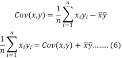
The variance of variable x can be expressed as-


Dividing equation (4) by n, we get-

From the equation (6), (7) and (8)-

Multiply (5) by , we get-

Subtracting equation (10) from equation (9), we get-


Since ‘b’ is the slope of the line of regression y on x and the line of regression passes through the point ( ), so that the equation of the line of regression of y on x is-


This is known as regression line of y on x.
Note-
 are the coefficients of regression.
2. 
Example: Two variables X and Y are given in the dataset below, find the two lines of regression.
x | 65 | 66 | 67 | 67 | 68 | 69 | 70 | 71 |
y | 66 | 68 | 65 | 69 | 74 | 73 | 72 | 70 |
Sol.
The two lines of regression can be expressed as-

And

x | y |  |  | Xy |
65 | 66 | 4225 | 4356 | 4290 |
66 | 68 | 4356 | 4624 | 4488 |
67 | 65 | 4489 | 4225 | 4355 |
67 | 69 | 4489 | 4761 | 4623 |
68 | 74 | 4624 | 5476 | 5032 |
69 | 73 | 4761 | 5329 | 5037 |
70 | 72 | 4900 | 5184 | 5040 |
71 | 70 | 5041 | 4900 | 4970 |
Sum = 543 | 557 | 36885 | 38855 | 37835 |
Now-

And

Standard deviation of x-


Similarly-


Correlation coefficient-


Put these values in regression line equation, we get
Regression line y on x-


Regression line x on y-


Regression line can also be find by the following method-
Example: Find the regression line of y on x for the given dataset.
X | 4.3 | 4.5 | 5.9 | 5.6 | 6.1 | 5.2 | 3.8 | 2.1 |
Y | 12.6 | 12.1 | 11.6 | 11.8 | 11.4 | 11.8 | 13.2 | 14.1 |
Sol.
Let y = a + bx is the line of regression of y on x, where ‘a’ and ‘b’ are given as-


We will make the following table-
x | y | Xy |  |
4.3 | 12.6 | 54.18 | 18.49 |
4.5 | 12.1 | 54.45 | 20.25 |
5.9 | 11.6 | 68.44 | 34.81 |
5.6 | 11.8 | 66.08 | 31.36 |
6.1 | 11.4 | 69.54 | 37.21 |
5.2 | 11.8 | 61.36 | 27.04 |
3.8 | 13.2 | 50.16 | 14.44 |
2.1 | 14.1 | 29.61 | 4.41 |
Sum = 37.5 | 98.6 | 453.82 | 188.01 |
Using the above equations we get-


On solving these both equations, we get-
a = 15.49 and b = -0.675
So that the regression line is –
y = 15.49 – 0.675x
Note – Standard error of predictions can be find by the formula given below-

Difference between regression and correlation-
1. Correlation is the linear relationship between two variables while regression is the average relationship between two or more variables.
2. There are only limited applications of correlation as it gives the strength of linear relationship while the regression is to predict the value of the dependent varibale for the given values of independent variables.
3. Correlation does not consider dependent and independent variables while regression consider one dependent variable and other indpendent variables.
Key takeaways-
- Karl Pearson’s coefficient of correlation-

2. Perfect Correlation: If two variables vary in such a way that their ratio is always constant, then the correlation is said to be perfect.
3. Short-cut method to calculate correlation coefficient-

4. Spearman’s rank correlation-

5. The variable which is used for prediction is called independent variable. It is known as predictor or regressor.
6. regression line is the best fit line which expresses the average relation between variables.
7. regression line of y on x.
A group of n individuals may be arranged in order to merit with respect to some characteristic. The same group would give different orders for different characteristics. Considering the order corresponding to two characteristics A and B for that group of individuals.
Let  be the ranks of the ith individuals in A and B respectively. Assuming that no two individuals are bracketed equal in either case, each of the variables taking the values 1,2,3,…,n, we have

If X,Y be the deviation of x, y from their means, then


Similarly 
Now let  so that


Hence the correlation coefficient between these variables is

This is called the rank correlation coefficient (Spearman’s rank corr) and is denoted by .
.
Spearman’s rank correlation-
When the ranks are given instead of the scores, then we use Spearman’s rank correlation to find out the correlation between the variables.
Spearman’s rank correlation coefficient can be defined as-

Example:
 | 1 | 6 | 5 | 10 | 3 | 2 | 4 | 9 | 7 | 8 |
 | 6 | 4 | 9 | 8 | 1 | 2 | 3 | 10 | 5 | 7 |
Solution:
If  , then


Hence
 nearly.
Example
Three judges A, B, C, give the following ranks. Find which pair of judges has common approach
A | 1 | 6 | 5 | 10 | 3 | 2 | 4 | 9 | 7 | 8 |
B | 3 | 5 | 8 | 4 | 7 | 10 | 2 | 1 | 6 | 9 |
C | 6 | 4 | 9 | 8 | 1 | 2 | 3 | 10 | 5 | 7 |
Solution: Here 
 | Ranks by  |  |   |   |   |  |  |  |
1 6 5 10 3 2 4 9 7 8 | 3 5 8 4 7 10 2 1 6 9 | 6 4 9 8 1 2 3 10 5 7 | -2 1 -3 6 -4 -8 2 8 1 -1 | -3 1 -1 -4 6 8 -1 -9 1 2 | 5 -2 4 -2 -2 0 -1 1 -2 -1 | 4 1 9 36 16 64 4 64 1 1 | 9 1 1 16 36 64 1 81 1 4 | 25 4 16 4 4 0 1 1 4 1 |
Total |
|
| 0 | 0 | 0 | 200 | 214 | 60 |

Since  is maximum, the pair of judges A and C have the nearest common approach.
Example: Compute the Spearman’s rank correlation coefficient of the dataset given below-
Person | A | B | C | D | E | F | G | H | I | J |
Rank in test-1 | 9 | 10 | 6 | 5 | 7 | 2 | 4 | 8 | 1 | 3 |
Rank in test-2 | 1 | 2 | 3 | 4 | 5 | 6 | 7 | 8 | 9 | 10 |
Solution
Person | Rank in test-1 | Rank in test-2 | d =  |  |
A | 9 | 1 | 8 | 64 |
B | 10 | 2 | 8 | 64 |
C | 6 | 3 | 3 | 9 |
D | 5 | 4 | 1 | 1 |
E | 7 | 5 | 2 | 4 |
F | 2 | 6 | -4 | 16 |
G | 4 | 7 | -3 | 9 |
H | 8 | 8 | 0 | 0 |
I | 1 | 9 | -8 | 64 |
J | 3 | 10 | -7 | 49 |
Sum |
|
|
| 280 |


Example: If X and Yare uncorrelated random variables,  the
the  of correlation between
  and
and 
Solution.
Let  and
and 
Then 
Now 
Similarly 
Now 


Also 


 (As
(As  and
and  are not correlated, we have
  )
)
Similarly 


Example 1 –
Test 1 | 8 | 7 | 9 | 5 | 1 |
Test 2 | 10 | 8 | 7 | 4 | 5 |
Solution
Here, highest value is taken as 1
Test 1 | Test 2 | Rank T1 | Rank T2 | d | d2 |
8 | 10 | 2 | 1 | 1 | 1 |
7 | 8 | 3 | 2 | 1 | 1 |
9 | 7 | 1 | 3 | -2 | 4 |
5 | 4 | 4 | 5 | -1 | 1 |
1 | 5 | 5 | 4 | 1 | 1 |
|
|
|
|
| 8 |

R = 1 – (6*8)/5(52 – 1) = 0.60
Example 2 -
Calculate Spearman rank-order correlation
English | 56 | 75 | 45 | 71 | 62 | 64 | 58 | 80 | 76 | 61 |
Maths | 66 | 70 | 40 | 60 | 65 | 56 | 59 | 77 | 67 | 63 |
Solution
Rank by taking the highest value or the lowest value as 1.
Here, highest value is taken as 1
English | Maths | Rank (English) | Rank (Math) | d | d2 |
56 | 66 | 9 | 4 | 5 | 25 |
75 | 70 | 3 | 2 | 1 | 1 |
45 | 40 | 10 | 10 | 0 | 0 |
71 | 60 | 4 | 7 | -3 | 9 |
62 | 65 | 6 | 5 | 1 | 1 |
64 | 56 | 5 | 9 | -4 | 16 |
58 | 59 | 8 | 8 | 0 | 0 |
80 | 77 | 1 | 1 | 0 | 0 |
76 | 67 | 2 | 3 | -1 | 1 |
61 | 63 | 7 | 6 | 1 | 1 |
|
|
|
|
| 54 |


R = 0.67
Therefore, this indicates a strong positive relationship between the ranks individuals obtained in the math and English exam.
Example 3 –
Find Spearman's rank correlation coefficient between X and Y for this set of data:
X | 13 | 20 | 22 | 18 | 19 | 11 | 10 | 15 |
Y | 17 | 19 | 23 | 16 | 20 | 10 | 11 | 18 |
Solution
X | Y | Rank X | Rank Y | d | d2 |
13 | 17 | 3 | 4 | -1 | 1 |
20 | 19 | 7 | 6 | 1 | 1 |
22 | 23 | 8 | 8 | 0 | 0 |
18 | 16 | 5 | 3 | 2 | 2 |
19 | 20 | 6 | 7 | -1 | 1 |
11 | 10 | 2 | 1 | 1 | 1 |
10 | 11 | 1 | 2 | -1 | 1 |
15 | 18 | 4 | 5 | -1 | 1 |
|
|
|
|
| 8 |
R = 

Example 4 – Calculation of equal ranks or tie ranks
Find Spearman's rank correlation coefficient:
Commerce | 15 | 20 | 28 | 12 | 40 | 60 | 20 | 80 |
Science | 40 | 30 | 50 | 30 | 20 | 10 | 30 | 60 |
Solution
C | S | Rank C | Rank S | d | d2 |
15 | 40 | 2 | 6 | -4 | 16 |
20 | 30 | 3.5 | 4 | -0.5 | 0.25 |
28 | 50 | 5 | 7 | -2 | 4 |
12 | 30 | 1 | 4 | -3 | 9 |
40 | 20 | 6 | 2 | 4 | 16 |
60 | 10 | 7 | 1 | 6 | 36 |
20 | 30 | 3.5 | 4 | -0.5 | 0.25 |
80 | 60 | 8 | 8 | 0 | 0 |
|
|
|
|
| 81.5 |

R = 1 – (6*81.5)/8(82 – 1) = 0.02
Example 5 –
X | 10 | 15 | 11 | 14 | 16 | 20 | 10 | 8 | 7 | 9 |
Y | 16 | 16 | 24 | 18 | 22 | 24 | 14 | 10 | 12 | 14 |
Solution
X | Y | Rank X | Rank Y | D | d2 |
10 | 16 | 6.5 | 5.5 | 1 | 1 |
15 | 16 | 3 | 5.5 | -2.5 | 6.25 |
11 | 24 | 5 | 1.5 | 3.5 | 12.25 |
14 | 18 | 4 | 4 | 0 | 0 |
16 | 22 | 2 | 3 | -1 | 1 |
20 | 24 | 1 | 1.5 | -0.5 | 0.25 |
10 | 14 | 6.5 | 7.5 | -1 | 1 |
8 | 10 | 9 | 10 | -1 | 1 |
7 | 12 | 10 | 9 | 1 | 1 |
9 | 14 | 8 | 7.5 | 0.5 | 0.25 |
|
|
|
|
| 24 |

R = 1 – (6*24)/10(102 – 1) = 0.85
The correlation between X and Y is positive and very high.
Operator E and  , Factorial notations
Definition:
Interpolation is a technique of estimating the value of a function for any intermediate value of the independent variable while the process of computing the value of the function outside the given range is called extrapolation.
Let  be a function of x.
The table given below gives corresponding values of y for different values of x.
X |  |  |
 | …. |  |
y= f(x) |  |  |  | …. |  |
The process of finding the values of y corresponding to any value of x which lies between  is called interpolation.
If the given function is a polynomial it is polynomial interpolation and given function is known as interpolating polynomial.
Note- The process of computing the value of the function outside the given range is called extrapolation.
Thus interpolation is the “art of reading between the lines of a table.”
Conditions for Interpolation
1) The function must be a polynomial of independent variable.
2) The function should be either increasing or decreasing function.
3) The value of the function should be increase or decrease uniformly.
Finite Difference
Let  be a function of x.The table given below gives corresponding values of y for different values of x.
X |  |  |
 | …. |  |
y= f(x) |  |  |  | …. |  |
|
|
|
|
|
|
There are three types of differences are useful-
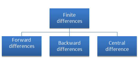
a) Forward Difference:
The  are called differences of y, denoted by
The symbol  is called the forward difference operator. Consider the forward difference table below:
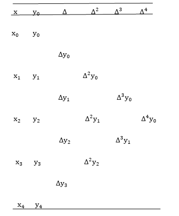
Where 
And  third forward difference so on.
b) Backward Difference:
The difference  are called first backward difference and is denoted by
  Consider the backward difference table below:
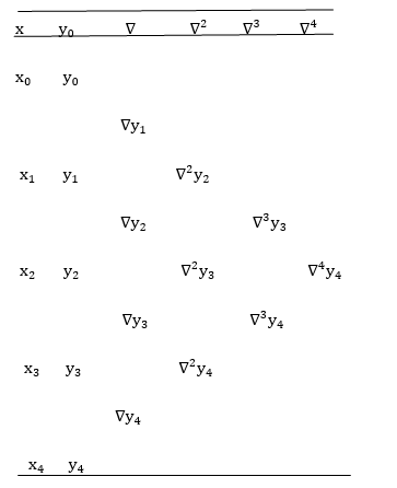
Where 
And  third backward differences so on.
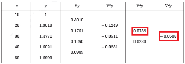
Example: Construct a backward difference table for y = log x, given-
X | 10 | 20 | 30 | 40 | 50 |
y | 1 | 1.3010 | 1.4771 | 1.6021 | 1.6990 |
Sol. The backward difference table will be-
Factorial:
The generalized nth power of a number x, denoted by  is defined as the product of n consecutive factors, the first of which is equal to x and each subsequent factor is h less than the preceding

Here h is some fixed constant  is also known as a “factorial function”. Here

Note- For h = 0, the generalized power coincides with the ordinary power

Lagrange’s Interpolation of polynomial:
Let  , be defined function we get
X |  |  |  | ….. |  |
f(x) |  |  |  | …… |  |
Where the interval is not necessarily equal. We assume f(x) is a polynomial od degree n. Then Lagrange’s interpolation formula is given by


Example1: Deduce Lagrange’s formula for interpolation. The observed values of a function are respectively 168,120,72 and 63 at the four position3,7,9 and 10 of the independent variable. What is the best estimate you can for the value of the function at the position6 of the independent variable.
We construct the table for the given data:
X | 3 | 6 | 7 | 9 | 10 |
Y=f(x) | 168 | ? | 120 | 72 | 63 |
We need to calculate for x = 6, we need f(6)=?
Here 
We get 
 By Lagrange’s interpolation formula, we have


Hence the estimated value for x=6 is 147.
Example2: By means of Lagrange’s formula, prove that

We construct the table:
X | 0 | 1 | 2 | 3 | 4 | 5 | 6 |
Y=f(x) |  |  |  |  |  |  |  |
Here x = 3, f(x)=?
 By Lagrange’s formula for interpolation


Hence proved.
Example3: find the polynomial of fifth degree from the following data
X | 0 | 1 | 3 | 5 | 6 | 9 |
Y=f(x) | -18 | 0 | 0 | -248 | 0 | 13104 |
Here 
We get 
 By Lagrange’s interpolation formula


Divided Difference:
In the case of interpolation, when the value of the arguments are not equi-spaced (unequal intervals) we use the class of differences called divided differences.
Definition: The difference which are defined by taking into consideration the change in the value of the argument are known as divided differences.
Let  be a function defined as
 |  |  | ……. |  |
 |  |  |
………… |  |
Where  are unequal i.e. it is case of unequal interval.
The first order divided differences are:


 And so on.
The second order divided difference is:


 And so on.
Similarly the nth order divided difference is:

With the help of these we construct the divided difference table:
X | f(x) |  |  |


 | 

 |

 |
  |
Newton’s Divided difference Formula:
Let  be a function defined as
 |  |  | ……. |  |
 |  |  |
………… |  |
Where  are unequal i.e. it is case of unequal interval.
 .
.
Example1: By means of Newton’s divided difference formula, find the values of  from the following table:
x | 4 | 5 | 7 | 10 | 11 | 13 |
f(x) | 48 | 100 | 294 | 900 | 1210 | 2028 |
We construct the divided difference table is given by:
x | f(x) | First order divide difference | Second order divide difference | Third order divide difference | Fourth order divide difference |
4
5
7
10
11
13 | 48
100
294
900
1210
2028 |


 |


 |


 |
0
0 |
By Newton’s Divided difference formula
 .
.

Now, putting  in above we get
 .
.


Example2: The following values of the function f(x) for values of x are given:

Find the value of  and also the value of x for which f(x) is maximum or minimum.
We construct the divide difference table:
x | f(x) | First order divide difference | Second order divide difference | Third order divide difference |
1
2
7
8 | 4
5
5
4 |


|


|
0 |
By Newton’s divided difference formula
 .
.


Putting  in above we get

For maximum and minimum of  , we have


Or 
Example3: Find a polynomial satisfied by  , by the use of Newton’s interpolation formula with divided difference.
x | -4 | -1 | 0 | 2 | 4 |
F(x) | 1245 | 33 | 5 | 9 | 1335 |
Here
We will construct the divided difference table:
x | F(x) | First order divided difference | Second order divided difference | Third order divided difference | Fourth order divided difference |
-4
-1
0
2
4 | 1245
33
5
9
1335 |


|


 |

 |
 |
By Newton’s divided difference formula
 .
.


This is the required polynomial.
References:
1. Higher Engineering Mathematics: B. S. Grewal
2. Applied Mathematics Volume I & II: J. N. Wartikar
3. Textbook of Engineering Mathematics: Bali, Iyenger (Laxmi Prakashan)