Unit - 2
Integral calculus-II
Curve tracing - An introduction
A picture explains more clearly than words and numbers. A curve which is the image of functional relationship gives us a lot information about the relation. We can get information analyzing the equation itself but the associated curve is often easy and understandable.
Let’s study about how to trace the curves of various equations in different forms like Cartesian, parametric and polar.
Important definitions for curve tracing
Here are some terms that we use in curve tracing:
1. Double point- when a curve passes two times through this point is known as double point.
2. Node- a double point at which two real tangents can be drawn.(tangents should not be coincide)
3. Cusp - a double point is a cusp when two tangents are coincide on it.
Asymptotes-
An asymptote of a curve of function y = f(x) is a line which does not intersect on the graph.
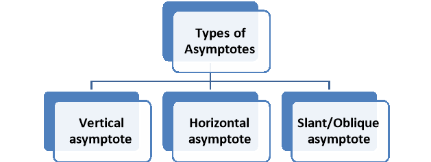
Types of asymptotes-
1. Vertical asymptote-
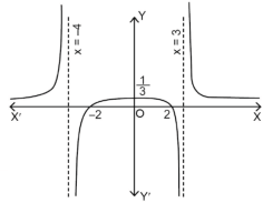
A line x = a which is straight is a vertical asymptote of the graph of the function y = f(x) if atleast one of the following condition does it follow-


Example: Determine the vertical asymptote of the function-

Sol. Here we have-

We can write the given function as-

We can notice here as x gets closer to 3 from the left, then the value of the function gets smaller, approaching -∞ and x gets closer 3 from the right, then the value of the function gets larger and approaches +∞.
So that x = 3 is a vertical asymptote same as x = -4 is another vertical asymptote.
2. Horizontal asymptote-
A line y = L is called horizontal asymptote to the curve of the function f(x)-
If f(x)→ L as x→∞ or as x→-∞
Example: Find the horizontal asymptote of the function-

Sol. In order to find the horizontal asymptote-
 =
= 
Hence the horizontal asymptote is y = 2.
Example: Find the horizontal asymptote of the function-

Sol. Find the limits-

And

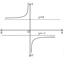
Hence the horizontal asymptotes are y = -1 and y = 5.
Figure will be as follows of the asymptotes of the given function-
3. Procedure to find the asymptotes parallel to axes of a polynomial function-
Theorem-
Suppose f(x , y) is a polynomial in x and y.
A straight line y = c is an asymptote of a curve f(x , y) = 0 if an only if y – c is a factor of the co-efficient of the highest power of x in f(x , y).
Example: Determine the asymptotes parallel to axes of the curve:
y² (x² - a²) = x
Sol. The given function can be written as-
y² (x² - a²) – x = 0
Asymptote parallel to x-axis-
Equating the coefficient of the highest power of x to zero, we get y² = 0 which means y = 0. This is an asymptote.
Asymptote parallel to y-axis-
Equating the coefficient of the highest power of x to zero, we get x² - a² = 0
Which gives x = ±a , that means x = +a , x = -a
So that these are the asymptotes.
4. Oblique asymptote or slant asymptote-
A straight line y = mx + c where m ≠ 0 will be an oblique/slant asymptote to the graph of the function ‘f’ if-

Note- the value of m can be find as-

And the value of c can be find as-
c = 
Example: Find the slant asymptotes of 
Sol. We have,

Which can be written as-

The value of ‘m’ will be-

=  =
= 
Now we can find ‘c’ as –
c =  =
=  =
= 
= 0
Hence the slant asymptotes are 
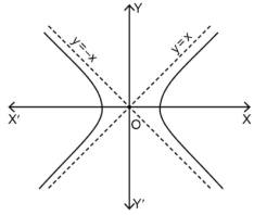
Example: Find the slant asymptote of the function f(x) = x +  .
.
Sol. Find the value of m-

Hence the y = x + c,
Now find c-

Here c must not be infinite.
So we can say that f does not have a slant asymptote at ∞.
Tracing a curve- Cartesian form
Let us the equation of a curve is f(x,y)=0 , now we will learn few steps to simplify tracing of this curve.
1. The first step to find out the region of the plane. For example no point in the curve x= y² in second and third quadrant as we will always get a positive value on x-axis. That means our curve will lie on first and fourth quadrant only.
2. The second step is to find out If the curve is symmetrical about any line or origin.
Some examples of symmetrical curves are as below-
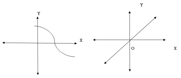
Symmetric about the x-axis Symmetric about origin
Steps to determine the symmetry of a curve:
1. If all the powers of x in function f(x,y)=0 are even, then f(x,y)= f(-x,y) and the curve is always symmetrical about y-axis. Similarly we can draw the conclusion about x-axis
2.If f(x,y)= 0 & f(-x,-y)= 0 , then the curve is symmetrical about the origin.
3. If the equation of the curve does not change when we interchange x and y then it is symmetrical about the line y= x
Let’s understand this with the help of following table-
Equation | Symmetry |
x⁴+y³+x⁶ = 0
y⁸+x⁹+y⁴ = 0
x⁴+ x²y²+y⁴ = 0
x²+y⁴ = 10 | About y-axis (even powers of x )
About x-axis( even powers of y)
About the origin as f(x,y)= 0 & f(-x,-y)= 0) About both axes as f(x,y)= f(-x,y), f(x,y)= f(x,-y) About the line y = x as f(x,y) = f(y,x)
About both axes ( even power of x and y) but not about y = x as f( x,y) is not equal to f(y ,x)+
|
4. The next step to determine the points where curve intersects the axes. If we put y = 0 in f(x,y)=0 and solve the equation, we get the points interecting on x-axis. Smilarly we get point on y- axis.
5. Now we try to locate the points for discontinuity of the function.
6. Calculate dy/dx to locate the portion where the curve is rising(dy/dx>0) or falling(dy/dx<0)
7. Calculate d²y/dx² to locate maxima and minima and the point of inflection
For maxima = dy/dx = 0, d²y/dx²<0 & for minima = dy/dx = 0, d²y/dx²>0
For point of inflection - d²y/dx² = 0
8. The next step is to find the asymptotes,
9. Another point to determine the singular point. The shape of the curve at these points generally more complex.
10. Finally plot the points as many as we can. Also try to draw tangents to the curve at some points(calculate the derivative). Now join the plotted point by a smooth curve.
Now we will understand curve tracing with some easy examples:
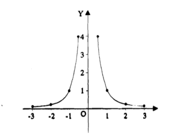
Example-: Trace the curve y = 1/x².
Sol.
As we can see y- coordinates of the curve can not be negative. So the curve must be above x-axis. The curve is also symmetric about y-axis so we can draw the graph only in single side.
Here, we will find the first and second derivatives-
So, dy/dx= -2/x³ and d²y/dx² = 6/ x⁴ , here dy/dx <0 for all x>0 so we can say that the function is non- increasing so the graph falls as we increase x.
Also second derivative is also non zero so there are no point of inflection.
Here the curve is x²y=1 (rewritten), here both the axes are asymptotes of the curve.
Here is the figure of the curve-:
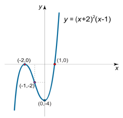
Example-2: Trace the curve y= (x+2)²(x-1).
Sol. Here first we check the slant asymptotes (there is no vertical asymptote)
So, p = 
= 
= 
= 
=  ) = +
) = +
Since p is infinity then the function has no slant asymptotes.
Now we will find the point of intersection with axes:
Y(0)= -4;
Put y(x)= 0, (x+2)²(x-1)= 0
We get by solving, X1= -2, x2= 1
Now calculate the first derivative,

Here we will find stationary point by putting first derivative equal to zero:
3x(x+2) = 0
X1 = 0, x2 = -2
X= -2 is maximum and x= 0 is minimum point.
The value of the function at these points will be:
Y= -4, 0
Now we will find second derivative:
Now, d²y/dx² = 6x+6,
So the function is strictly upward for:
X<-1,
And strictly downward for
x>-1,
Hence x= -1 is the inflection point
We get y(-1)= -2
Here is the figure of curve:
Tracing a curve- parametric form
Before we start tracing curves of the equations in parametric form, here first we understand the definition of parametric equations:
Parametric equations:
If x and y are the continuous functions of “t” on an interval I , then the equations:
x = x(t)
And
y= y(t)
Are called parametric equations and t is called the parameter.
Now let’s understand how to trace the curves in parametric by examples:
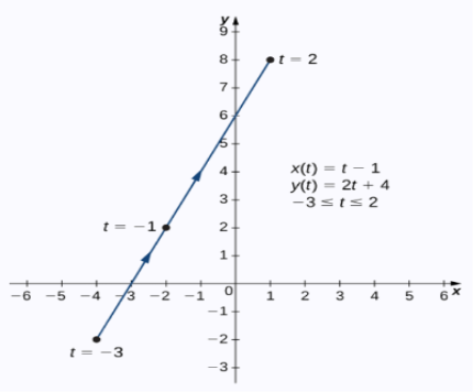
Example1: trace the curve of the following parametric equations:
x(t) = t-1 , y(t) = 2t+4 -3<
Sol. Here we will create the table for t, x(t) and y(t), t is independent variable in both case,
t | x(t) | y(t) |
-3 | -4 | -2 |
-2 | -3 | 0 |
-1 | -2 | 2 |
0 | -1 | 4 |
1 | 0 | 6 |
2 | 1 | 8 |
Here value of t lies between -3 to 2.
By plotting these set of point we get a curve as below.
Arrows in the graph indicates the orientation of the graph.
Tracing a curve- polar form
To trace the polar curve r = f ( we follow the following steps:
1. Symmetry –
(a) if the equation is an even function of  , then the curve is symmetrical about the initial line.
(b) if the equation is an even function of r, then the curve is symmetrical about the origin/
(C ) If the equation remains same if we change  by -
by - and r by –r then the curve is symmetric about the line through the pole and perpendicular to the initial line.
2. Region- Find the reason for  for which r is defined and real
3. Table- make table for the values of r determined by  .
.
4. Angle  -
-  is the angle between the radius vector and tangent to the curve;
 =
=  )
)
Then angle  =
=  +
+ , tangents to the curve can be determined by angle
5. Asymptotes- find the asymptotes of the curve.
Now we will understand of tracing of polar equations by an example:
Example: Trace the curve r = a(1+ cos .
.
Sol. Here we can see clearly cos = cos(-
 ), hence the curve is symmetric about initial line.
Since -1 , the curve lies inside the circle r = 2a
 = -asin
 , when 0
 , thus r decreases as
  increases in the interval 0 to
 |
0 |
 |
 |
r |
2a |
A |
0 |
 = - cot (
 ) = tan(
 +
+  ), this shows the angle between r and
  and the tangent is 0 or
  according to
  0 or
0 or  . Hence the line joining a point on the curve to the origin is orthogonal to the tangent when
 = 0 and coincides with
From the above results, we can easily draw the graph above the initial line
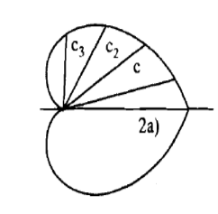
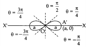
Example-2: Trace the curve  .
.
Sol. Symmetry about initial line- Put r = 0, 
Hence the straight line  are the tangents to the curve at the pole.
Values of ‘r’ as  changes from 0 to π-
Table for the values of ‘r’-
 |  |  |
 |  |  |
 | 0 | 0 |
 |  | Imaginary |
 | 0 | 0 |
 |  |  |
 |  |  |
Here according to the table the curve does not exist for the value lying between  to
to 
The figure will be as follows of the curve-
Key takeaways-
1. An asymptote of a curve of function y = f(x) is a line which does not intersect on the graph.
2. Double point- when a curve passes two times through this point is known as double point.
3. Node- a double point at which two real tangents can be drawn.(tangents should not be coincide)
4. Cusp - a double point is a cusp when two tangents are coincide on it.
There is wide range of definite integrals such as, from geometric applications to physical world problems.
We will study about these applications one by one-
(1) Area between the curves-
Suppose we want to find out the area between y = f(x) and y = g(x) on interval [a,b] such that f(x) ≥ g(x). See the figure
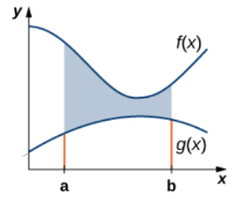
Let the area between the two curve is A, then
A = 
Lets do some examples,
Example-1: find the area under the curves where f(x) = x+4 and g(x) = 3 – x/2 over the interval [1,4]
Sol. Here limits are given a = 1 , b = 4,
We know that, area under the curve,
A = 
= 
= 
= 
= (16 – 7/4) = 57/4
So that the area of the region is 57/4 unit square.
Example-2: find the area under the curves where y = x and y = x + 1, x = 2 and y-axis.
Sol. When we draw the graph, curve does not meet, but depend on two vertical lines,
Here boundary is [0 , 2]
Area under the curve,
A = 
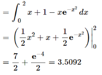
So that the area under the curve is 3.2092 unit square.
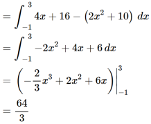
Example-2: Determine the area under the curves y = 2x² + 10 and y = 4x + 16.
Sol. Here we will find out the intersection, which are the boundaries of the curve,
2x² + 10 = 4x + 16
2x² - 4x – 6 = 0
2 (x + 1) ( x – 3 ) = 0
We get, x = -1 and x = 3,
We know that, Area under the curve,
A = 
(2) Average function value-
We can use definite integrals to find out the average value of a function.
The average value of a function over the interval [a , b] is given by the following expression ,
f( avg.) = 
Example-1: find the average value of the function f(x) = x³ over the interval[0,1].
Sol. We know that
f( avg.) = 
=  =
=  = 1 / 4
Example-2: find the average value of f(x) = cosx over the interval [0 , 𝛑/2]
Sol. We know that,
f( avg.) = 
Put the values, we get

(3) Work-
This one is the easiest use of definite integral
We know that work done, when a constant force F is applied to move the object over a distance d.
W = Fd
Now suppose that the force at any point x is F(x), the the work done by to move the object from x = a to x = b is,
W = 
Example-1: Find the work done on a spring when we compress it from its natural length of 1m to the 0.75m, if the spring constant k = 16 N / m.
Sol. The force is given by,
F =16x
Here we start to compress it at x = 0 and finish at x= 0.25 from its natural length.
So we take lower limit and upper limit 0 and 0.25 respectively.
We know that,
W = 
= 
= 0.5 N.m
Example-2: A force of 1200 N compresses a spring from its natural length of 18 cm to a length of 16 cm. How much work is done in compressing it from 16 cm to 14 cm?
Sol. Here,
F = kx
So that,
1200 = 2k
K = 600 N/cm
In that case,
F = 600x
We know that,
W = 
W =  , which gives
W = 3600 N.cm
Length of plane curves
We can use definite integrals to find out the length of the arc of a curve.
Suppose a rocket launched along a parabolic path and if we are interested to find the length of the how much distance has rocket covered the we can use the concept of arc length of curve.
Let f(x) be a smooth function over the interval [a,b]. Then the arc length of the proportion of f(x) from point (a,f(a)) to the point (b, f(b)) is given by,
Length of Arc =
Note - Smooth functions- functions which are continuous derivative are called smooth.
Example-1: let f(x) = 2 x³/² ,then calculate the arc length of the graph over interval [ 0 , 1].
Sol. Here we can find its first derivative
f’(x) = 3 x¹/²
Such that,
[f’(x)]² = 9x
Then we know that,
Length of Arc =
= 
Now,
Let u = 1 + 9x , then du = 9 dx , when x = 0 then u = 1 and x = 1 then u = 10,
So,
= 
= 
= 1/9 ×2/3 ×  = 2.268 units
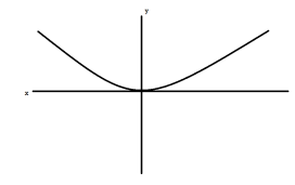
Example-2: suppose a wire hanging on two poles follows the curve,
f(x) = a cosh(x/a)
Find the length of the wire.
Sol. We will find the first derivative of f(x),
f’(x) = sinh(x/a)
The curve of f(x) will look like,
Hence the curve os symmetric, we will measure the length of one side first,
The limits on one side will be, 0 to b
We know that
Length of Arc =
Put f’(x) = sinh(x/a), we get
Length of Arc =
Use the identity,

= 
= 
We get on solving,
Asinh(b/a)
On both sides, the length of the curve will be,
2 a sinh(b/a)
Example_3: Find the length of f(x) = x between x = 2 and x = 3.
Sol. The derivative of f(x) will be,
f’(x) = 1
And we know that,
Length of Arc =
So that,
Length of Arc =
= 
On solving the integral, we get
= (3 – 2) =
=  .
.
Key takeaways-
- f( avg.) =

- W =

- Length of Arc =

- Functions which are continuous derivative are called smooth.
Area in Cartesian coordinates-
Example-1: Find the area enclosed by two curves using double integration.
y = 2 – x and y² = 2 (2 – x)
Sol. Let,
y = 2 – x ………………..(1)
And y² = 2 (2 – x) ………………..(2)
On solving eq. (1) and (2)
We get the intersection points (2,0) and (0,2) ,
We know that,
Area = 
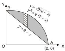
Here we will find the area as below,
Area = 


Which gives,
= ( - 4 + 4 /2 ) + 8 / 3 = 2 / 3.
Example-2: Find the area between the parabola y ² = 4ax and another parabola x² = 4ay.
Sol. Let,
y² = 4ax ………………..(1)
And
x² = 4ay…………………..(2)
Then if we solve these equations, we get the values of points where these two curves intersect
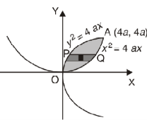
x varies from y²/4a to  and y varies from o to 4a,
Now using the conceot of double integral,
Area = 


Area in polar coordinates-
Example-3: Find the area lying inside the cardioid r = a(1+cosθ) and outside the circle r = a, by using double integration.
Sol. We have,
r = a(1+cosθ) …………………….(1)
And
r = a ……………………………….(2)
On solving these equations by eliminating r , we get
a(1+cosθ) = a
(1+cosθ) = 1
Cosθ = 0
Here a θ varies from – π/2 to π/2
Limit of r will be a and 1+cosθ)
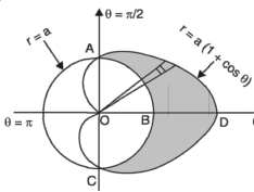
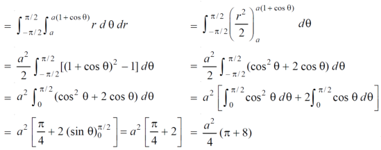
Which is the required area.
Example-4: Find the are lying inside a cardioid r = 1 + cosθ and ouside the parabola r(1 + cosθ) = 1.
Sol. Let,
r = 1 + cosθ ……………………..(1)
r(1 + cosθ) = 1……………………..(2)
Solving these equestions , we get
(1 + cosθ )(1 + cosθ ) = 1
(1 + cosθ )² = 1
1 + cosθ = 1
Cosθ = 0
θ = ±π / 2
So that, limits of r are,
1 + cosθ and 1 / 1 + cosθ
The area can be founded as below,

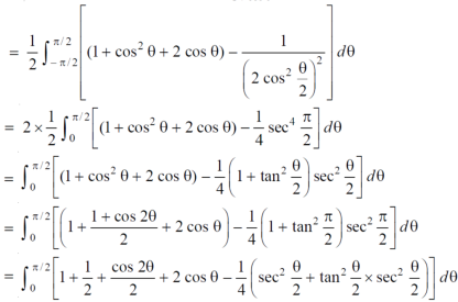

Double integrals as volumes
Suppose we have a curve y = f(x) is revolved about an axis , then a solid is generated , now we need to find out the volume of the solid generated
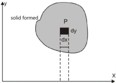
The formula for volume of the solid generated about x-axis,

Example-1: Calculate the volume generated by the revolution of a cardioid,
r = a ( 1 – cosθ) about its axis
Sol. Here, r = a ( 1 – cosθ)
Volume =


=

Which is the volume of generated by cardioid.
Example-2: Find the volume generated by revolving a circle x ² + y² = 4 about the line x= 3.
Sol. We know that,
Volume = 
Here , PQ = 3 – x,
= 


The volume is 24π².
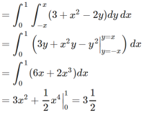
Example-3: Calculate the volume under the surface z = 3 + x² - 2y over the region R defined as 0≤ x ≤ 1 and -x ≤ y ≤ x
Sol. The is a double integral of z = 3 + x² - 2y over the region R .
Volume will be,
Key takeaways-
The formula for volume of the solid generated about x-axis,

Areas and volumes of revolutions
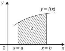
The volume of revolution (V) is obtained by rotating area A through one revolution about the x-axis is given by-

Suppose the curve x = f(y) is rotated  about y-axis between the limits y = c and y = d, then the volume generated V, is given by-

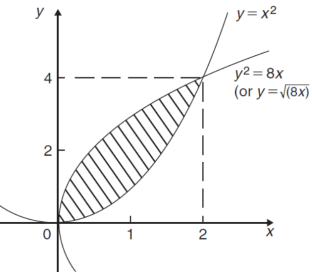
Example-1: Find the area enclosed by the curves  and if the area is rotated
  about the x-axis then determine the volume of the solid of revolution.
Sol. We know that, at the point of intersection the coordinates of the curve are equal. So that first we will find the point of intersection-


We get,
x = 0 and x = 2
The curve of the given equations will look like as follows-
Then,
The area of the shaded region will be-
A = 
So that the area will be 8/3 square unit.
The volume will be
= (volume produced by revolving  – (volume produced by revolving
= 
Method of cylindrical shells-
Let f(x) be a continuous and positive function. Define R as the region bounded above by the graph f(x), below by the x-axis, on the left by the line x = a and on the right x = b, then the volume of the solid of revolution formed by revolving R around the y-axis is given by

Example-2: Find the volume of the solid of revolution formed by revolving R around y-axis of the function f(x) = 1/x over the interval [1 , 3].
Sol. The graph of the function f(x) = 1/x will look like-
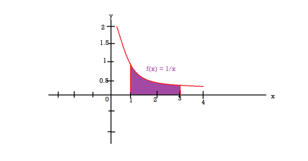
The volume of the solid of revolution generated by revolving R(violet region) about the y-axis over the interval [1 , 3]
Then the volume of the solid will be-


Example-3: Find the volume of the solid of revolution formed by revolving R around y-axis of the function f(x) = 2x - x² over the interval [0 , 2].
Sol. The graph of the function f(x) = 2x - x² will be-
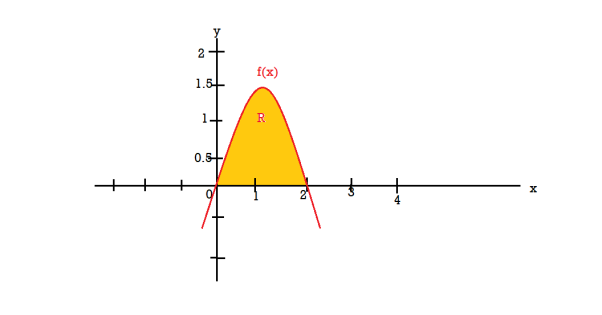
The volume of the solid is given by-


= 
Area of surfaces of revolution
Suppose we have a curve y = f(x) and if we revolve this curve around x – axis then the area formed is known as surface area of revolution.
Let f(x) be a non-negative smooth function over the interval[ [ a , b] , then the surface area of the surface of revolution formed by revolving the graph of f(x) around x-axis is given by,
S = 
Example-1: Find the surface of the surface generated by revolving the graph f(x) =  over the interval [1,4] around x-axis.
Sol. The graph of the function will look like
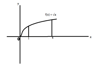
f(x) =  then f’(x) = 1/2 (
(f’(x))² = 1/4x
Then,
S = 
S = 
S =  ,
,
Let u =  , then du = dx, when x = 1 , u = 5/4 and when x = 4 , u = 17/4,
This will give,
 =
= 
On solving the integral we get,
 = 30.84 (approx.)
Example-1: find the surface of the surface generated by revolving the graph g(y) =  over the interval [0,2] around y-axis.
Sol.
Hint - use formula
S = 
Ans. = 24.118
References:
1. Higher Engineering Mathematics: B. S. Grewal
2. Applied Mathematics Volume I & II: J. N. Wartikar
3. Textbook of Engineering Mathematics: Bali, Iyenger (Laxmi Prakashan)