Unit - 3

Mathematical expectations and probability distributions

3.1 Discrete Random Variable: Review of discrete random variable

Random variables

It is a real valued function which assigns a real number to each sample point in the sample space.

A random variable X is a function defined on the sample space 5 of an experiment S of an experiment. Its value are real numbers. For every number a the probability

With which X assumes a is defined. Similarly for any interval l the probability

With which X assumes any value in I is defined.

Example:

Tossing a fair coin thrice then-

Sample Space(S) = {HHH, HHT, HTH, THH, HTT, THT, TTH, TTT}

Roll a dice

Sample Space(S) = {1,2,3,4,5,6}

A random variable is a real-valued function whose domain is a set of possible outcomes of a random experiment and range is a sub-set of the set of real numbers and has the following properties:

i) Each particular value of the random variable can be assigned some probability

Ii) Uniting all the probabilities associated with all the different values of the random variable gives the value 1.

A random variable is denoted by X, Y, Z etc.

For example if a random experiment E consists of tossing a pair of dice, the sum X of the two numbers which turn up have the value 2,3,4,…12 depending on chance. Then X is a random variable 

Probability mass function-

Let X be a r.v. Which takes the values and let P[X = ] = p(. This function p(xi), i =1,2, … defined for the values assumed by X is called probability mass function of X satisfying p(xi) ≥0 and

Example: A random variable x has the following probability distribution-

Then find-

1. Value of c.

2. P[X≤3]

3. P[1 < X <4]

Sol.

We know that for the given probability distribution-

So that-

2.

P[X ≤ 3] = P[X = 3] + P[X = 2] + P[X =1] + P[X = 0]

= 2c + c + c + 0 = 4c = 4 × 1/8 = ½

3.

Discrete random variable-

A random variable is said to be discrete if it has either a finite or a countable number of values. Countable number of values means the values which can be arranged in a sequence.

Note- if a random variable takes a finite set of values it is called discrete and if if a random variable takes an infinite number of uncountable values it is called continuous variable.

Discrete probability distributions-

Let X be a discrete variate which is the outcome of some experiments. If the probability that X takes the values of x is , then-

Where-

1.

2.

The set of values with their probabilities makes a discrete probability distribution of the discrete random variable X.

Probability distribution of a random variable X can be exhibited as follows-

X			and so on
P(x)

Example: Find the probability distribution of the number of heads when three coins are tossed simultaneously.

Sol.

Let be the number of heads in the toss of three coins

The sample space will be-

{HHH, HHT, HTH, THH, HTT, THT, TTH, TTT}

Here variable X can take the values 0, 1, 2, 3 with the following probabilities-

P[X= 0] = P[TTT] = 1/8

P[X = 1] = P [HTT, THH, TTH] = 3/8

P[X = 2] = P[HHT, HTH, THH] = 3/8

P[X = 3] = P[HHH] = 1/8

Hence the probability distribution of X will be-

X
P(x)

Example: For the following probability distribution of a discrete random variable X,

Find-

1. The value of c.

2. P[1<x<4]

Sol,

1. We know that-

So that-

0 + c + c + 2c + 3c + c = 1

8c = 1

Then c = 1/8

Now, 2. P[1<x<4] = P[X = 2] + P[X = 3] = c + 2c = 3c = 3× 1/8 = 3/8

Probability density function

Probability density function (PDF) is a arithmetical appearance which gives a probability distribution for a discrete random variable as opposite to a continuous random variable. The difference among a discrete random variable is that we check an exact value of the variable. Like, the value for the variable, a stock worth, only goes two decimal points outside the decimal (Example 32.22), while a continuous variable have an countless number of values (Example 32.22564879…).

When the PDF is graphically characterized, the area under the curve will show the interval in which the variable will decline. The total area in this interval of the graph equals the probability of a discrete random variable happening. More exactly, since the absolute prospect of a continuous random variable taking on any exact value is zero owing to the endless set of possible values existing, the value of a PDF can be used to determine the likelihood of a random variable dropping within a exact range of values.

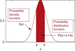
Example: The probability density function of a variable X is

(i)                Find

(ii)             What will be e minimum value of k so that

Solution

(i) If X is a random variable then

(iii)           Thus minimum value of k=1/30.

Example: A random variate X has the following probability function

x	0	1	2	3	4	5	6	7
P (x)	0	k	2k	2k	3k

(i)                Find the value of the k.

(ii)            

Solution. (i) If X is a random variable then

3.2 Probability function and Distribution function

Continuous probability distribution

When a variate X takes every value in an interval it gives rise to continuous distribution of X. The distribution defined by the vidiots like heights or weights are continuous distributions.

A major conceptual difference however exist between discrete and continuous probabilities. When thinking in discrete terms the probability associated with an event is meaningful. With continuous events however where the number of events is infinitely large, the probability that a specific event will occur is practically zero. For this reason continuous probability statements on must be worth did some work differently from discrete ones. Instead of finding the probability that x equals some value, we find the probability of x falling in a small interval.

Thus the probability distribution of a continuous variate x is defined by a function f (x) such that the probability of the variate x falling in the small interval Symbolically it can be expressed as Thus f (x) is called the probability density function and then continuous curve y = f(x) is called the probability of curve.

The range of the variable may be finite or infinite. But even when the range is finite, it is convenient to consider it as infinite by opposing the density function to be zero outside the given range. Thus if f (x) =(x) be the density function denoted for the variate x in the interval (a,b), then it can be written as

The density function f (x) is always positive and (i.e. the total area under the probability curve and the the x-axis is is unity which corresponds to the requirements that the total probability of happening of an event is unity).

Distribution function

If

Then F(x) is defined as the commutative distribution function or simply the distribution function the continuous variate X. It is the probability that the value of the variate X will be ≤x. The graph of F(x) in this case is as shown in figure 26.3 (b).

The distribution function F (x) has the following properties

(i)               

(ii)             

(iii)          

(iv)            P(a ≤x ≤b)= = =F (b) – F (a).

Example.

(i)                Is the function defined as follows a density function.

(ii)             If so determine the probability that the variate having this density will fall in the interval (1.2).

(iii)          Also find the cumulative probability function F (2)?

Solution. (i) f (x) is clearly ≥0 for every x in (1,2) and

Hence the function f (x) satisfies the requirements for a density function.

(ii)Required probability =

This probability is equal to the shaded area in figure 26.3 (a).

(iii)Cumulative probability function F(2)

Which is shown in figure

Example: Show that the following function can be defined as a density function and then find .

Sol.

Here

So that, the function can be defined as a density function.

Now.

Example: Let X be a continuous random variable with PDF given by

If , find the CDF of Y.

Solution. First we note that , we have

Thus,
 

Example: Let X be a continuous random variable with PDF

Find .

Solution. We have

Key takeaways-

1. A random variable is said to be discrete if it has either a finite or a countable number of values. Countable number of values means the values which can be arranged in a sequence.

2.

Where-

1.

3.3 Mathematical expectation

Let a random variable X has a probability distribution which assumes the values say with their associated probabilities then the mathematical expectation can be defined as-

The expected value of a random variable X is written as E(X).

Expected value for a continuous random variable is

Example: If a random variable X has the following probability distribution in tabular form then what will be the expected value of X.

Sol.

We know that-

So that-

Example: Find the expectations of the number of an unbiased die when thrown.

Sol. Let X be a random variable which represents the number on a die when thrown.

X can take the values-

1, 2, 3, 4, 5, 6

With

P[X = 1] = P[X = 2] = P[X = 3] = P[X = 4] = P[X = 5] = P[X = 6] = 1/6

The distribution table will be-

Hence the expectation of number on the die thrown is-

So that-

3.4 Variance and Standard deviation

Standard deviation:

It is defined as the positive square root of the arithmetic mean of the square of the deviation of the given values from their arithmetic mean. It is denoted by the symbol .

Where is A.M of the distribution . We have more formulae to calculate the standard deviation.

….                  

In frequency distribution from, we put where H is generally taken as width of class interval

Shortcut formula to calculate standard deviation-

The square of the standard deviation is called known as a variance.

Example-1: Compute the variance and standard deviation.

Sol.

Class	Mid-value (x)	Frequency (f)
0-10	5	3	1470.924
10-20	15	5	737.250
20-30	25	7	32.1441
30-40	35	9	555.606
40-50	45	4	1275.504
Sum			4071.428

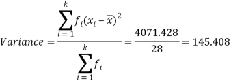
Then standard deviation,

Example-2: Calculate the standard deviation of the following frequency distribution-

Sol.

Weight	Item (f)	X	d = x – 67	f.d
60 – 62	5	61	-6	-30	180
63 – 65	18	64	-3	-54	162
66 – 68	42	67	0	0	0
69 – 71	27	70	3	81	243
72 – 74	8	73	6	48	288
Total	100			45	873

Example: Calculate S.D for the following distribution.

Solution:

Wages earned C.I	Mid value	Frequency
52	5	5	-2	-10	20
153	15	9	-1	-9	9
25	25	15	0	0	0
35	35	12	1	12	12
45	45	10	2	20	40
55	55	3	3	9	27
Total	-

Using formula,

3.5 Moments, Moment generating function

Moments-

The r’th moment of a variable x about the mean is denoted by and defined as-

The r’th moment of a variable x about any point ‘a’ will be-

Relationship between moments about mean and moment about any point-

When two variables are related in such a way that change in the value of one variable affects the value of the other variable, then these two variables are said to be correlated and there is correlation between two variables.

Example- Height and weight of the persons of a group.

The correlation is said to be perfect correlation if two variables vary in such a way that their ratio is constant always.

Variance of a sum

One of the applications of covariance is finding the variance of a sum of several random variables. In particular, if Z = X + Y, then

                                                     Var (Z) =Cov (Z,Z)

More generally, for a, bR we conclude

Variance

Consider two random variables X and Y with the following PMFs

                      (3.3)

                           (3.4)

Note that EX =EY = 0. Although both random variables have the same mean value, their distribution is completely different. Y is always equal to its mean of 0, while X is IDA 100 or -100, quite far from its mean value. The variance is a measure of how spread out the distribution of a random variable is. Here the variance of Y is quite small since its distribution is concentrated value. Why the variance of X will be larger since its distribution is more spread out.

The variance of a random variable X with mean , is defined as

By definition the variance of X is the average value of Since ≥0, the variance is always larger than or equal to zero. A large value of the variance means that is often large, so X often X value far from its mean. This means that the distribution is very spread out. On the other hand a low variance means that the distribution is concentrated around its average.

Note that if we did not square the difference between X and its mean the result would be zero. That is

X is sometimes below its average and sometimes above its average. Thus is sometimes negative and sometimes positive but on average it is zero.

To compute , note that we need to find the expected value of , so we can use LOTUS. In particular we can write

For example, for X and Y defined in equations 3.3 and 3.4 we have

As we expect, X has a very large variance while Var (Y) = 0

Note that Var (X) has a different unit than X. For example, if X is measured in metres then Var(X) is in .to solve this issue we define another measure called the standard deviation usually shown as which is simply the square root of variance.

The standard deviation of a random variable X is defined as

The standard deviation of X has the same unit as X. For X and Y defined in equations 3.3 and 3.4 we have

Here is a useful formula for computing the variance.

Computational formula for the variance

To prove it note that

Note that for a given random variable X, is just a constant real number. Thus so we have

Equation 3.5 is equally easier to work with compared to . To use this equation we can find using LOTUS.

And then subtract to obtain the variance.

Example. I roll a fair die and let X be the resulting number. Find EX, Var(X), and

Solution. We have   and for k = 1,2,…,6. Thus we have

Thus ,

Theorem

For random variable X and real number a and b

Proof. If

From equation 3.6, we conclude that, for standard deviation, . We mentioned that variance is NOT a linear operation. But there is a very important case, in which variance behave like a linear operation and that is when we look at sum of independent random variables,

Theorem

If are independent random variables and , then

Example. If Binomial (n, p) find Var (X).

Solution. We know that we can write a Binomial (n, p) random variable as the sum of n independent Bernoulli (p) random variable, i.e.

If Bernoulli (p) then its variance is

Problem. If , find Var (X).

Solution. We already know , thus Var (X). You can find directly using LOTUS, however, it is a little easier to find E [X (X-1)] first. In particular using LOTUS we have

S

So we have . Thus, and we conclude

Key takeaways-

1.    

2.    

3.    

4.    

5.     For random variable X and real number a and b

6.     If are independent random variables and , then

3.6 Probability Distributions: Binomial distribution

BINOMIAL DISTRIBUTION

To find the probability of the happening of an event once, twice, thrice,…r times ….exactly in n trails.

Let the probability of the happening of an event A in one trial be p and its probability of not happening be 1 – p – q.

We assume that there are n trials and the happening of the event A is r times and its not happening is n – r times.

This may be shown as follows

AA……A                                 

r times                                       n – r times                          (1)

A indicates its happening its failure and P (A) =p and P (

We see that (1) has the probability

Pp…p qq….q=

r times              n-r times                                                       (2)

Clearly (1) is merely one order of arranging r A’S.

The probability of (1) =Number of different arrangements of r A’s and (n-r)’s

The number of different arrangements of r A’s and (n-r)’s

Probability of the happening of an event r times =

If r = 0, probability of happening of an event 0 times

If r = 1,probability of happening of an event 1 times

If r = 2,probability of happening of an event 2 times

If r = 3,probability of happening of an event 3 times and so on.

These terms are clearly the successive terms in the expansion of

Hence it is called Binomial Distribution.

Binomial distribution-

A discrete random variable X is said to be follow the binomial distribution with parameter n and p.

The probability of happening of an event r times exactly in n trials is-

Example: A die is thrown 8 times then find the probability that 3 will show-

1. Exactly 2 times

2. At least 7 times

3. At least once

Sol.

As we know that-

Then-

1. Probability of getting 3 exactly 2 times will be-

2.     Probability of getting 3 at least 7 or 8 times will be-

3.     Probability of getting 3 at least once or (1 or 2 or 3 or 4 or 5 or 6 or 7 or 8 times)-

= P(1) +P(2) +P(3) +P(4) + P(5) + P(6) +P(7) +P(8)

= 1 – P(0) = 1 -

= 1 –

Example: If the percentage of failure in a test is 20. If six students appear in the test, then what will be the probability that at least five students will pass the test?

Sol.

Here

Then the probability of at least five students will pass the test-

= P(5) +P(6) =

Example: Find mean and variance of a binomial distribution with p = 1/4 and n = 10.

Sol.

Here

Mean = np =

Variance = npq =

Example: If a dice is rolled thrice. A success is getting 1 or 6 on a roll. Find the mean variance of the number of success.

Sol.

Here n = 3 , p = 1/3 and q = 2/3

Mean = np = 1

And variance = npq = 2/3

Example. If on an average one ship in every ten is wrecked. Find the probability that out of 5 ships expected to arrive, 4 at least we will arrive safely.

Solution. Out of 10 ships one ship is wrecked.

I.e. nine ships out of 10 ships are safe, P (safety) =

P (at least 4 ships out of 5 are safe) = P (4 or 5) = P (4) + P(5)

Example. The overall percentage of failures in a certain examination is 20. If 6 candidates appear in the examination what is the probability that at least five pass the examination?

Solution. Probability of failures = 20%

Probability of (P) =

Probability of at least 5 pass = P(5 or 6)

Example. The probability that a man aged 60 will live to be 70 is 0.65. What is the probability that out of 10 men, now 60, at least seven will live to be 70?

Solution. The probability that a man aged 60 will live to be 70

Number of men= n = 10

Probability that at least 7 men will live to 70 = (7 or 8 or 9 or 10)

= P (7)+ P(8)+ P(9) + P(10) =

Example. Assuming that 20% of the population of a city are literate so that the chance of an individual being literate is and assuming that hundred investigators each take 10 individuals to see whether they are illiterate, how many investigators would you expect to report 3 or less were literate.

Solution.

Required number of investigators = 0.879126118× 100 =87.9126118

= 88 approximate

Mean or binomial distribution

Successors r	Frequency f	Rf
0		0
1
2		n(n-1)
3
…..	……	….
n

Since,

STANDARD DEVIATION OF BINOMIAL DISTRIBUTION

Successors r	Frequency f
0		0
1
2		2n(n-1)
3
…..	……	….
n

We know that           (1)

r is the deviation of items (successes) from 0.

Putting these values in (1) we have

Hence for the binomial distribution, Mean

Example. A die is tossed thrice. A success is getting 1 or 6 on a TOSS. Find the mean and variance of the number of successes.

Solution.

RECURRENCE RELATION FOR THE BINOMIAL DISTRIBUTION

By Binomial Distribution

On dividing (2) by (1) , we get

3.7 Poisson distribution

Poisson distribution is a limiting case of binomial distribution under certain conditions listed below-

1. n, the number of trials are infinitely large.

2. p, the probability of success for each trial is very small.

3. Np is finite quantity say

A random variable X is said to be follow Poisson distribution if it has the following probability mass function-

Moments of Poisson distribution-

1. First moment about origin- which Is known as mean.

2. Second moment about origin-

3. Third moment about origin-

4. Fourth moment about origin-

Note-

1. Poisson distribution is always positively skewed distribution.

2. Mean and variance of Poisson dist. Are always equal

For Poisson distribution-

Mean = np

Variance = npq

μ3 = npq (q – p)

μ4 = npq[ 1 + 3 pq (n-2)] = npq[1 + 3npq – 6pq]

Example: If cars arriving at workshop follow the Poisson distribution. If the average number of cars arrivals during a specified period of an hour is 2.

Find the probabilities that during the given hour-

1. No car arrive

2. At least two cars arrive.

Sol.

Here the average of car arrivals is - 2

So that mean = 2

Let X be the number of cars arriving during the given  hour,

By using Poisson distribution, we get-

So that the required probability-

1. P [no car will arrive] = P [X = x] =

2. P [At least two cars will arrive] = P [X≥2] = P [X =2] + P [X = 3] + ……….

              = 1 - P [[X =1] + P [X =0]]

Example: If the probability that a vaccine given to the patients shows bad reaction is 0.001, then find the probability that out of 2000 patients-

1. Exactly 3 patients

2. More than 2 patients

3. No patient

Will show bad reaction.

Sol.

Here p = 0.001 and number of patients (n) = 2000

Then

By using Poisson distribution, we get-

1. Probability that exactly 3 patients show bad reaction is-

2. Probability that more than 2 patients show bad reaction-

3. Probability that no patient shows bad reaction-

Example: If a book has 600 pages and it has 40 printing mistakes. Assume that these mistakes are randomly distributed and x the number of mistakes per page follow Poisson distribution.

What is the probability that there will not be any mistake if 10 pages selected at random?

Sol.

Here

We get by using Poisson distribution-

Then-

3.8 Normal distribution

The concept of normal distribution was given by English mathematician Abraham De Moivre in 1733 but the concrete theory was given by Karl Gauss that is why sometime normal distribution is called Gaussian distribution.

Normal distribution is a continuous distribution. It is derived as the limiting form of the Binomial distribution for large values of n and p and q are not very small.

The normal distribution is given by the equation

    (1)

Where = mean, = standard deviation, =3.14159…e=2.71828…

On substitution in (1) we get      (2)

Here mean = 0, standard deviation = 1

(2) is known as standard form of normal distribution.

Note-

1. If a random variable X follows normal distribution with mean and variance then we can write it as- X

2. If X , then is called standard normal variate with mean 0 and standard deviation 1.

3. The probability density function of standard normal variate Z is given as-

Where

Graph of a normal probability function-

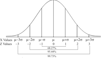
The curve look like bell-shaped curve. The top of the bell is exactly above the mean.

If the value of standard deviation is large then curve tends to flatten out and for small standard deviation it has sharp peak.

This is one of the most important probability distributions in statistical analysis.

MEAN FOR NORMAL DISTRIBUTION

Mean         [Putting

STANDARD DEVIATION FOR NORMAL DISTRIBUTION

Put,

MEDIAN OF THE NORMAL DISTRIBUTION

If a is the median then it divides the total area into two equal halves so that

Where,

Suppose mean, then

Thus,

Similarly, when mean, we have a =

Thus, median = mean =

MEA DEVIATION ABOUT THE MEAN

Mean deviation

MODE OF THE NORMAL DISTRIBUTION

We know that mode is the value of the variate x for which f (x) is maximum. Thus by differential calculus f (x) is maximum if and

Where,

Thus mode is and model ordinate =

NORMAL CURVE

Let us show binomial distribution graphically. The probabilities of heads in 1 tosses are

. It is shown in the given figure.

If the variates (head here) are treated as if they were continuous, the required probability curve will be a normal curve as shown in the above figure by dotted lines.

Properties of the normal curve

1. The curve is symmetrical about the y- axis. The mean, median and mode coincide at the origin.
2. The curve is drawn, if mean (origin of x) and standard deviation are given. The value of can be calculated from the fact that the area of the curve must be equal to the total number of observations.
3. y decreases rapidly as x increases numerically. The curve extends to infinity on either side of the origin.
4. (a)

AREA UNDER THE NORMAL CURVE

By taking the standard normal curve is formed.

The total area under this curve is 1. The area under the curve is divided into two equal parts by z = 0. Left hand side area and right hand side area to z = 0 is 0.5. The area between the ordinate z = 0.

Example. On a final examination in mathematics, the mean was 72, and the standard deviation was 15. Determine the standard scores of students receiving graders.

(a)  60

(b)  93

(c)  72

Solution. (a)

(b)

(c)

Example. Find the area under the normal curve in each of the cases

(a)  Z = 0 and z = 1.2

(b)  Z = -0.68 and z = 0

(c)  Z = -0.46 and z = -2.21

(d)  Z = 0.81 and z = 1.94

(e)  To the left of z = -0.6

(f)    Right of z = -1.28

Solution. (a) Area between Z = 0 and z = 1.2 =0.3849

(b)Area between z = 0 and z = -0.68 = 0.2518

(c)Required area = (Area between z = 0 and z = 2.21) + (Area between z = 0 and z =-0.46)\

= (Area between z = 0 and z = 2.21)+ (Area between z = 0 and z = 0.46)

=0.4865 + 0.1772 = 0.6637

(d)Required area = (Area between z = 0 and z = 1.+-(Area between z = 0 and z = 0.81)

= 0.4738-0.2910=0.1828

(e) Required area = 0.5-(Area between z = 0 and z = 0.6)

                                 = 0.5-0.2257=0.2743

(f)Required area = (Area between z = 0 and z = -1.28)+0.5

                               = 0.3997+0.5

                               = 0.8997

Example. The mean inside diameter of a sample of 200 washers produced by a machine is 0.0502 cm and the standard deviation is 0.005 cm. The purpose for which these washers are intended allows a maximum tolerance in the diameter of 0.496 to 0.508 cm, otherwise the washers are considered defective. Determine the percentage of defective washers produced by the machine assuming the diameters are normally distributed.

Solution.

Area for non – defective washers = Area between z = -1.2

And z = +1.2

=2 Area between z = 0 and z = 1.2

=2 (0.3849)-0.7698=76.98%

Percentage of defective washers = 100-76.98=23.02%

Example. A manufacturer knows from experience that the resistance of resistors he produces is normal with mean and standard deviation . What percentage of resistors will have resistance between 98 ohms and 102 ohms?

Solution. ,

Area between

                                = (Area between z = 0 and z = +1)

                           = 2 (Area between z = 0 and z = +1)=2 0.3413 = 0.6826

Percentage of resistors having resistance between 98 ohms and 102 ohms = 68.26

Example. In a normal distribution, 31% of the items are 45 and 8% are over 64. Find the mean and standard deviation of the distribution.

Solution. Let be the mean and the S.D.

If x = 45,

If x = 64,

Area between 0 and

[From the table, for the area 0.19, z = 0.496)

Area between z = 0 and z =

(from the table for area 0.42, z = 1.405)

Solving (1) and (2) we get

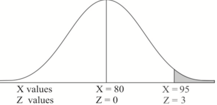
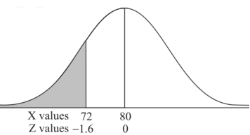
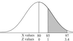
Example: If a random variable X is normally distributed with mean 80 and standard deviation 5, then find-

1. P[X > 95]

2. P[X < 72]

3. P [85 < X <97]

[Note- use the table- area under the normal curve]

Sol.

The standard normal variate is –

Now-

1. X = 95,

So that-

2. X = 72,

So that-

3. X = 85,

X = 97,

So that-

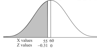
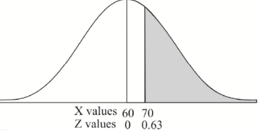
Example: In a company the mean weight of 1000 employees is 60kg and standard deviation is 16kg.

Find the number of employees having their weights-

1. Less than 55kg.

2. More than 70kg.

3. Between 45kg and 65kg.

Sol. Suppose X be a normal variate = the weight of employees.

Here mean 60kg and S.D. = 16kg

X

Then we know that-

We get from the data,

Now-

1. For X = 55,

So that-

P[X < 55] = P[Z < - 0.31] = P[Z > 0.31]

= 0.5 – P[0 < Z < 0.31]

= 0.5 – 0.1217

=0.3783

2. For X = 70,

So that-

P[X > 70] = P[Z > 0.63]

= 0.5 – P[0 < Z < 0.63]

= 0.5 – 0.2357 = 0.2643

3. For X = 45,

For X = 65,

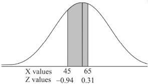
Hence the number of employees having weights between 45kg and 65kg-

Example: The mean inside diameter of a sample of 200 washers produced by a machine is 0.0502 cm and the standard deviation is 0.005 cm. The purpose for which these washers are intended allows a maximum tolerance in the diameter of 0.496 to 0.508 cm, otherwise the washers are considered defective. Determine the percentage of defective washers produced by the machine, assuming the diameters are normally distributed.

Sol.

Here-

And

Area for non-defective washers = area between z = -1.2 to +1.2

= 2 area between z = 0 and z = 1.2

= 2 × 0.3849 = 0.7698 = 76.98%

Then percent of defective washers = 100 – 76.98 = 23.02 %

Example: The life of electric bulbs is normally distributed with mean 8 months and standard deviation 2 months.

If 5000 electric bulbs are issued how many bulbs should be expected to need replacement after 12 months?

[Given that P (z ≥ 2) = 0. 0228]

Sol.

Here mean (μ) = 8 and standard deviation = 2

Number of bulbs = 5000

Total months (X) = 12

We know that-

Area (z ≥ 2) = 0.0228

Number of electric bulbs whose life is more than 12 months ( Z> 12)

= 5000 × 0.0228 = 114

Therefore replacement after 12 months = 5000 – 114 = 4886 electric bulbs

3.9 Exponential distribution

Many scientific experiments involve the measurement of the duration of time X between an initial point of time and the occurrence of some phenomenon of interest. For example X is the life time of a light bulb which is turned on and left until it burns out. The continuous random variable X having the probability density function

Where, the rate λ signifies the Normal amount of events in single time.

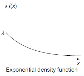
Is said to have an exponential distribution. Here the only parameter of the distribution is λ which is greater than zero. This distribution, also known as the negative exponential distribution, is a special case of the gamma distribution (with r = 1). Examples of random variables modeled as exponential are-

a. (inter-arrival) time between two successive job arrivals

b. Duration of telephone calls

c. Life time (or time to failure) of a component or a product

d. Service time at a server in a queue

e. Time required for repair of a component

The mean value is μ = . The median of the exponential distribution is m = , and the variance is shown by .

Note: Both the mean and standard deviation of the exponential distribution are equal to

Example: Let the mileage (in thousands of miles) of a particular tyre be a random variable X having the probability density

f(x) =

Find the probability that one of these tyres will last

(a) at most 10,000 miles

(b) anywhere from 16,000 to 24,000 miles

(c) at least 30,000 miles.

(d) Find the mean

(e) Find the variance of the given probability density function.

Sol:

(a) Probability that a tyre will last almost

10,000 miles

= P(X ≤ 10) =

=

= . .

= 1 – e- ½ = 0.3934

b.

c.

d. Mean = μ =

=

μ = 20 = 1/λ

e.

Variance = σ2 =

Consider

=  0 + 2. 20 . μ = 2.20.20 = 2.202

Then

Example: The length of time for one person to be served at a cafeteria is a random variable X having an exponential distribution with a mean of 4 minutes. Find the probability that a person is served in less than 3 minutes on at least 4 of the next 6 days.

Sol:

The probability that a person is served at a cafeteria in less than 3 minutes is

P(T < 3) = 1 – P(T

Since the mean μ = 1/ λ = 4 or λ = 1/4 , the exponential

Distribution is ¼

Now

P(T < 3) = 1 – P(T ≥ 3) = 1 -

P(T < 3) = 1 – ¼ .

Let X represent the number of days on which a person is served in less than 3 minutes. Then using the binomial distribution, the probability that a person is served in less than 3 minutes on at least 4 of the next 6 days is

P(X ≥ 4) =

References:

1. E. Kreyszig, “Advanced Engineering Mathematics”, John Wiley & Sons, 2006.
2. P. G. Hoel, S. C. Port And C. J. Stone, “Introduction To Probability Theory”, Universal Book Stall, 2003.
3. S. Ross, “A First Course in Probability”, Pearson Education India, 2002.
4. W. Feller, “An Introduction To Probability Theory and Its Applications”, Vol. 1, Wiley, 1968.
5. N.P. Bali and M. Goyal, “A Text Book of Engineering Mathematics”, Laxmi Publications, 2010.
6. B.S. Grewal, “Higher Engineering Mathematics”, Khanna Publishers, 2000.