Unit - 4
Statistical techniques
Correlation:
So far we have confined our attention to the analysis of observation on a single variable. There are, however, many phenomena where the changes in one variable are related to the changes in the other variable. For instance, the yield of crop varies with the amount of rainfall, the price of a commodity increases with the reduction in its supply and so on. Such a simultaneous variation, i.e., when the changes in one variable are associated or followed by change in the other, is called correlation. Such a data connecting two variables is called bivariate population.
If an increase (or decrease) in the values of one variable corresponds to an increase (or decrease) in the other, the correlation is said to be positive. If the increase (or decrease) in one corresponds to the decrease (or increase) in other, the correlation is said to be negative. If there is no relationship indicated between the variables, they are said to be independent or uncorrelated.
When two variables are related in such a way that change in the value of one variable affects the value of the other variable, then these two variables are said to be correlated and there is correlation between two variables.
Example- Height and weight of the persons of a group.
The correlation is said to be perfect correlation if two variables vary in such a way that their ratio is constant always.
Types of correlation:
According to the direction of change in variables there are two types of correlation
1. Positive Correlation
2. Negative Correlation
1. Positive Correlation:
Correlation between two variables is said to be positive if the values of the variables deviate in the same direction i.e. if the values of one variable increase (or decrease) then the values of other variable also increase (or decrease). For example:
1. Heights and weights of group of persons;
2. House hold income and expenditure;
3. Amount of rainfall and yield of crops
2. Negative Correlation:
Correlation between two variables is said to be negative if the values of variables deviate in opposite direction i.e. if the values of one variable increase(or decrease) then the values of other variable decrease (or increase). Some examples of negative correlations are correlation between
1. Volume and pressure of perfect gas;
2. Price and demand of goods;
3. Literacy and poverty in a country
Scatter diagram-
Scatter diagram is a statistical tool for determining the potentiality of correlation between dependent variable and independent variable. Scatter diagram does not tell about exact relationship between two variables but it indicates whether they are correlated or not.
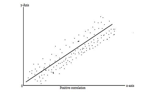
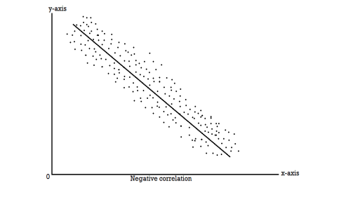
To obtain a measure of relationship between the two variables, we plot their corresponding values on the graph, taking one of the variables along the x-axis and the other along the y-axis.
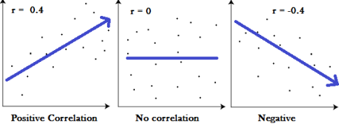
Correlation measures the nature and strength of relationship between two variables. Correlation lies between +1 to -1. A correlation of +1 indicates a perfect positive correlation between two variables. A zero correlation indicates that there is no relationship between the variables. A correlation of -1 indicates a perfect negative correlation.
Definition-
“Correlation analysis deals with the association between two or more variables.” —Simpson and Kafka
“Correlation is an analysis of the co-variation between two variables.” —A.M. Tuttle
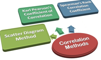
Methods of computing coefficient of correlation
- Scatter diagram method-
It is the simplest method to study correlation between two variables. The correlations of two variables are plotted in the graph in the form of dots thereby obtaining as many points as the number of observations. The degree of correlation is ascertained by looking at the scattered points over the charts.
The more the points plotted are scattered over the chart, the lesser is the degree of correlation between the variables. The more the points plotted are closer to the line, the higher is the degree of correlation. The degree of correlation is denoted by “r”.
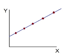
- Perfect positive correlation (r = +1) – All the points plotted on the straight line rising from left to right
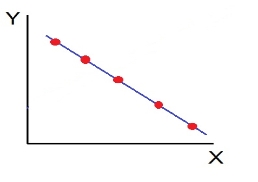
- Perfect negative correlation (r=-1) – all the points plotted on the straight line falling from left to right
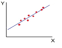
- High Degree of +Ve Correlation (r= + High): all the points plotted close to the straight line rising from left to right
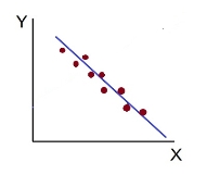
- High Degree of –Ve Correlation (r= – High) - all the points plotted close to the straight line falling from left to right.
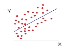
- Low degree of +Ve Correlation (r= + Low): all the points are highly scattered to the straight line rising from left to right
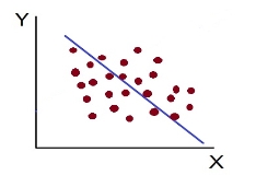
- Low Degree of –Ve Correlation (r= - Low): all the points are highly scattered to the straight line falling from left to right
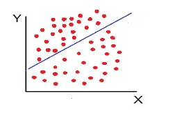
- No Correlation (r= 0) – all the points are scattered over the graph and do not show any pattern
2. Karl Pearson’s coefficient of correlation:
Coefficient of correlation measures the intensity or degree of linear relationship between two variables. It was given by British Biometrician Karl Pearson (1867-1936).
Karl Pearson’s Coefficient of Correlation is widely used mathematical method is used to calculate the degree and direction of the relationship between linear related variables. The coefficient of correlation is denoted by “r”.
If X and Y are two random variables then correlation coefficient between Xand Y is denoted by r and defined as-
Karl Pearson’s coefficient of correlation-

Here-  and
and 

Note-
1. Correlation coefficient always lies between -1 and +1.
2. Correlation coefficient is independent of change of origin and scale.
3. If the two variables are independent then correlation coefficient between them is zero.
Correlation coefficient | Type of correlation |
+1 | Perfect positive correlation |
-1 | Perfect negative correlation |
0.25 | Weak positive correlation |
0.75 | Strong positive correlation |
-0.25 | Weak negative correlation |
-0.75 | Strong negative correlation |
0 | No correlation |
Example: Find the correlation coefficient between Age and weight of the following data-
Age | 30 | 44 | 45 | 43 | 34 | 44 |
Weight | 56 | 55 | 60 | 64 | 62 | 63 |
Sol.
x | Y |  |  |  |  | (   |
30 | 56 | -10 | 100 | -4 | 16 | 40 |
44 | 55 | 4 | 16 | -5 | 25 | -20 |
45 | 60 | 5 | 25 | 0 | 0 | 0 |
43 | 64 | 3 | 9 | 4 | 16 | 12 |
34 | 62 | -6 | 36 | 2 | 4 | -12 |
44 | 63 | 4 | 16 | 3 | 9 | 12 |
Sum= 240 |
360 |
0 |
202 |
0 |
70
|
32 |
Karl Pearson’s coefficient of correlation-

Here the correlation coefficient is 0.27.which is the positive correlation (weak positive correlation), this indicates that the as age increases, the weight also increase.
Short-cut method to calculate correlation coefficient-

Here,


Example: Find the correlation coefficient between the values X and Y of the dataset given below by using short-cut method-
X | 10 | 20 | 30 | 40 | 50 |
Y | 90 | 85 | 80 | 60 | 45 |
Sol.
X | Y |  |  |  |  |  |
10 | 90 | -20 | 400 | 20 | 400 | -400 |
20 | 85 | -10 | 100 | 15 | 225 | -150 |
30 | 80 | 0 | 0 | 10 | 100 | 0 |
40 | 60 | 10 | 100 | -10 | 100 | -100 |
50 | 45 | 20 | 400 | -25 | 625 | -500 |
Sum = 150 |
360 |
0 |
1000 |
10 |
1450 |
-1150 |
Short-cut method to calculate correlation coefficient-


Example
Psychological tests of intelligence and of engineering ability were applied to 10 students. Here is a record of ungrouped data showing intelligence ratio (I.R) and engineering ratio (E.R). Calculate the co-efficient of correlation.
Student | A | B | C | D | E | F | G | H | I | J |
I.R | 105 | 104 | 102 | 101 | 99 | 98 | 96 | 92 | 93 | 92 |
E.R | 101 | 103 | 100 | 98 | 96 | 104 | 92 | 94 | 97 | 94 |
Solution:
We construct the following table:
Student | Intelligence ratio x 
| Engineering ratio y  | X2 | Y2 | XY |
A B C D E F G H I J | 100 6 104 5 102 3 101 2 100 1 99 0 98 -1 96 -3 93 -6 92 -7 | 101 3 103 5 100 2 98 0 95 -3 96 -2 104 6 92 -6 97 -1 94 -4 | 36 25 9 4 1 0 1 9 36 49 | 9 25 4 0 9 4 36 36 1 16 | 18 25 6 0 -3 0 -6 18 6 28 |
Total | 990 0 | 980 0 | 170 | 140 | 92 |
From this table, mean of  i.e.,
i.e.,  and mean of
  , i.e.,

Substituting these values in the formula (1), we have

Other examples:
Example-1-Compute Pearsons coefficient of correlation between advertisement cost and sales as per the data given below:
Advertisement cost | 39 | 65 | 62 | 90 | 82 | 75 | 25 | 98 | 36 | 78 |
Sales | 47 | 53 | 58 | 86 | 62 | 68 | 60 | 91 | 51 | 84 |
Solution
X | Y |  |  |  |  | (X -  |
39 | 47 | -26 | 676 | -19 | 361 | 494 |
65 | 53 | 0 | 0 | -13 | 169 | 0 |
62 | 58 | -3 | 9 | -8 | 64 | 24s |
90 | 86 | 25 | 625 | 20 | 400 | 500 |
82 | 62 | 17 | 289 | -4 | 16 | -68 |
75 | 68 | 10 | 100 | 2 | 4 | 20 |
25 | 60 | -40 | 1600 | -6 | 36 | 240 |
98 | 91 | 33 | 1089 | 25 | 625 | 825 |
36 | 51 | -29 | 841 | -15 | 225 | 435 |
78 | 84 | 13 | 169 | 18 | 324 | 234 |
650 | 660 |
| 5398 |
| 2224 | 2704 |
|
|
|
|
|
|
|

r = (2704)/√5398 √2224 = (2704)/(73.2*47.15) = 0.78
Thus Correlation coefficient is positively correlated
Example 2
Compute correlation coefficient from the following data
Hours of sleep (X) | Test scores (Y) |
8 | 81 |
8 | 80 |
6 | 75 |
5 | 65 |
7 | 91 |
6 | 80 |
X | Y |  |  |  |  | (X -  |
8 | 81 | 1.3 | 1.8 | 2.3 | 5.4 | 3.1 |
8 | 80 | 1.3 | 1.8 | 1.3 | 1.8 | 1.8 |
6 | 75 | -0.7 | 0.4 | -3.7 | 13.4 | 2.4 |
5 | 65 | -1.7 | 2.8 | -13.7 | 186.8 | 22.8 |
7 | 91 | 0.3 | 0.1 | 12.3 | 152.1 | 4.1 |
6 | 80 | -0.7 | 0.4 | 1.3 | 1.8 | -0.9 |
40 | 472 |
| 7 |
| 361 | 33 |
 = 40/6 =6.7
 = 472/6 = 78.7

r = (33)/√7 √361 = (33)/(2.64*19) = 0.66
Thus Correlation coefficient is positively correlated
Example 3
Calculate coefficient of correlation between X and Y series using Karl pearson shortcut method
X | 14 | 12 | 14 | 16 | 16 | 17 | 16 | 15 |
Y | 13 | 11 | 10 | 15 | 15 | 9 | 14 | 17 |
Solution
Let assumed mean for X = 15, assumed mean for Y = 14
X | Y | Dx | Dx2 | Dy | Dy2 | Dxdy |
14 | 13 | -1.0 | 1.0 | -1.0 | 1.0 | 1.0 |
12 | 11 | -3.0 | 9.0 | -3.0 | 9.0 | 9.0 |
14 | 10 | -1.0 | 1.0 | -4.0 | 16.0 | 4.0 |
16 | 15 | 1.0 | 1.0 | 1.0 | 1.0 | 1.0 |
16 | 15 | 1.0 | 1.0 | 1.0 | 1.0 | 1.0 |
17 | 9 | 2.0 | 4.0 | -5.0 | 25.0 | -10.0 |
16 | 14 | 1 | 1 | 0 | 0 | 0 |
15 | 17 | 0 | 0 | 3 | 9 | 0 |
120 | 104 | 0 | 18 | -8 | 62 | 6 |


r = 48/√144*√432 = 0.19
3. Spearman’s rank correlation coefficient
A group of n individuals may be arranged in order to merit with respect to some characteristic. The same group would give different orders for different characteristics. Considering the order corresponding to two characteristics A and B for that group of individuals.
Let xi, yi be the ranks of the ith individuals in A and B respectively. Assuming that no two individuals are bracketed equal in either case, each of the variables taking the values 1,2,3,…,n, we have

If X,Y be the deviation of x, y from their means, then


Similarly 
Now let di = xi - yi so that di = (xi -  - (yi -
  = Xi - Yi


Hence the correlation coefficient between these variables is

This is called the rank correlation coefficient (Spearman’s rank corr) and is denoted by ρ.
Spearman’s rank correlation-
When the ranks are given instead of the scores, then we use Spearman’s rank correlation to find out the correlation between the variables.
Spearman’s rank correlation coefficient can be defined as-

Example:
 | 1 | 6 | 5 | 10 | 3 | 2 | 4 | 9 | 7 | 8 |
 | 6 | 4 | 9 | 8 | 1 | 2 | 3 | 10 | 5 | 7 |
Solution:
If di = xi - yi, then di = -5, 2, -4, 2, 2, 0, 1, -1, 2, 1

Hence

Example
Three judges A, B, C, give the following ranks. Find which pair of judges has common approach
A | 1 | 6 | 5 | 10 | 3 | 2 | 4 | 9 | 7 | 8 |
B | 3 | 5 | 8 | 4 | 7 | 10 | 2 | 1 | 6 | 9 |
C | 6 | 4 | 9 | 8 | 1 | 2 | 3 | 10 | 5 | 7 |
Solution:Here 
 | Ranks by  |  |  |  |  |  |  |  |
1 6 5 10 3 2 4 9 7 8 | 3 5 8 4 7 10 2 1 6 9 | 6 4 9 8 1 2 3 10 5 7 | -2 1 -3 6 -4 -8 2 8 1 -1 | -3 1 -1 -4 6 8 -1 -9 1 2 | 5 -2 4 -2 -2 0 -1 1 -2 -1 | 4 1 9 36 16 64 4 64 1 1 | 9 1 1 16 36 64 1 81 1 4 | 25 4 16 4 4 0 1 1 4 1 |
Total |
|
| 0 | 0 | 0 | 200 | 214 | 60 |


Since  is maximum, the pair of judges A and C have the nearest common approach.
Example: Compute the Spearman’s rank correlation coefficient of the dataset given below-
Person | A | B | C | D | E | F | G | H | I | J |
Rank in test-1 | 9 | 10 | 6 | 5 | 7 | 2 | 4 | 8 | 1 | 3 |
Rank in test-2 | 1 | 2 | 3 | 4 | 5 | 6 | 7 | 8 | 9 | 10 |
Solution
Person | Rank in test-1 | Rank in test-2 | d =  |  |
A | 9 | 1 | 8 | 64 |
B | 10 | 2 | 8 | 64 |
C | 6 | 3 | 3 | 9 |
D | 5 | 4 | 1 | 1 |
E | 7 | 5 | 2 | 4 |
F | 2 | 6 | -4 | 16 |
G | 4 | 7 | -3 | 9 |
H | 8 | 8 | 0 | 0 |
I | 1 | 9 | -8 | 64 |
J | 3 | 10 | -7 | 49 |
Sum |
|
|
| 280 |


Example: If X and Yare uncorrelated random variables,  the
the  of correlation between
  and
and 
Solution.
Let  and
and 
Then 
Now 
Similarly 
Now 


Also 


 (As
(As  and
and  are not correlated, we have
  )
)
Similarly 


Example 1 –
Test 1 | 8 | 7 | 9 | 5 | 1 |
Test 2 | 10 | 8 | 7 | 4 | 5 |
Solution
Here, highest value is taken as 1
Test 1 | Test 2 | Rank T1 | Rank T2 | d | d2 |
8 | 10 | 2 | 1 | 1 | 1 |
7 | 8 | 3 | 2 | 1 | 1 |
9 | 7 | 1 | 3 | -2 | 4 |
5 | 4 | 4 | 5 | -1 | 1 |
1 | 5 | 5 | 4 | 1 | 1 |
|
|
|
|
| 8 |

R = 1 – (6*8)/5(52 – 1) = 0.60
Example 2 -
Calculate Spearman rank-order correlation
English | 56 | 75 | 45 | 71 | 62 | 64 | 58 | 80 | 76 | 61 |
Maths | 66 | 70 | 40 | 60 | 65 | 56 | 59 | 77 | 67 | 63 |
Solution
Rank by taking the highest value or the lowest value as 1.
Here, highest value is taken as 1
English | Maths | Rank (English) | Rank (Math) | d | d2 |
56 | 66 | 9 | 4 | 5 | 25 |
75 | 70 | 3 | 2 | 1 | 1 |
45 | 40 | 10 | 10 | 0 | 0 |
71 | 60 | 4 | 7 | -3 | 9 |
62 | 65 | 6 | 5 | 1 | 1 |
64 | 56 | 5 | 9 | -4 | 16 |
58 | 59 | 8 | 8 | 0 | 0 |
80 | 77 | 1 | 1 | 0 | 0 |
76 | 67 | 2 | 3 | -1 | 1 |
61 | 63 | 7 | 6 | 1 | 1 |
|
|
|
|
| 54 |


R = 0.67
Therefore, this indicates a strong positive relationship between the ranks individuals obtained in the math and English exam.
Example 3 –
Find Spearman's rank correlation coefficient between X and Y for this set of data:
X | 13 | 20 | 22 | 18 | 19 | 11 | 10 | 15 |
Y | 17 | 19 | 23 | 16 | 20 | 10 | 11 | 18 |
Solution
X | Y | Rank X | Rank Y | d | d2 |
13 | 17 | 3 | 4 | -1 | 1 |
20 | 19 | 7 | 6 | 1 | 1 |
22 | 23 | 8 | 8 | 0 | 0 |
18 | 16 | 5 | 3 | 2 | 2 |
19 | 20 | 6 | 7 | -1 | 1 |
11 | 10 | 2 | 1 | 1 | 1 |
10 | 11 | 1 | 2 | -1 | 1 |
15 | 18 | 4 | 5 | -1 | 1 |
|
|
|
|
| 8 |
R = 

Example 4 – Calculation of equal ranks or tie ranks
Find Spearman's rank correlation coefficient:
Commerce | 15 | 20 | 28 | 12 | 40 | 60 | 20 | 80 |
Science | 40 | 30 | 50 | 30 | 20 | 10 | 30 | 60 |
Solution
C | S | Rank C | Rank S | d | d2 |
15 | 40 | 2 | 6 | -4 | 16 |
20 | 30 | 3.5 | 4 | -0.5 | 0.25 |
28 | 50 | 5 | 7 | -2 | 4 |
12 | 30 | 1 | 4 | -3 | 9 |
40 | 20 | 6 | 2 | 4 | 16 |
60 | 10 | 7 | 1 | 6 | 36 |
20 | 30 | 3.5 | 4 | -0.5 | 0.25 |
80 | 60 | 8 | 8 | 0 | 0 |
|
|
|
|
| 81.5 |

R = 1 – (6*81.5)/8(82 – 1) = 0.02
Example 5 –
X | 10 | 15 | 11 | 14 | 16 | 20 | 10 | 8 | 7 | 9 |
Y | 16 | 16 | 24 | 18 | 22 | 24 | 14 | 10 | 12 | 14 |
Solution
X | Y | Rank X | Rank Y | D | d2 |
10 | 16 | 6.5 | 5.5 | 1 | 1 |
15 | 16 | 3 | 5.5 | -2.5 | 6.25 |
11 | 24 | 5 | 1.5 | 3.5 | 12.25 |
14 | 18 | 4 | 4 | 0 | 0 |
16 | 22 | 2 | 3 | -1 | 1 |
20 | 24 | 1 | 1.5 | -0.5 | 0.25 |
10 | 14 | 6.5 | 7.5 | -1 | 1 |
8 | 10 | 9 | 10 | -1 | 1 |
7 | 12 | 10 | 9 | 1 | 1 |
9 | 14 | 8 | 7.5 | 0.5 | 0.25 |
|
|
|
|
| 24 |

R = 1 – (6*24)/10(102 – 1) = 0.85
The correlation between X and Y is positive and very high.
Key takeaways:
- Positive Correlation: Correlation between two variables is said to be positive if the values of the variables deviate in the same direction
- Negative Correlation: Correlation between two variables is said to be negative if the values of variables deviate in opposite direction
- Karl Pearson’s coefficient of correlation:

4. Correlation coefficient always lies between -1 and +1.
5. If the two variables are independent then correlation coefficient between them is zero
6. Short-cut method to calculate correlation coefficient-

7. Spearman’s rank correlation-

Regression Analysis
As the correlation analysis studies the nature and extent of interrelationship between the two variables X and Y, regression analysis helps us to estimate or approximate the value of one variable when we know the value of other variable. Therefore, we can define the ‘Regression’ as the estimation (prediction) of one variable from the other variable when they are correlated to each other. e.g., We can estimate the Demand of the commodity if we know it’s Price.
Why are there two regressions?
When the variables X and Y are correlated there are two possibilities,
(i)Variable X depends on variable y. In this case we can find the value of x if know the value of y. This is called regression of x on  .
.
(ii)Variable  depends on variable X. We can find the value of y if know the value of X. This is called regression of y on x. Hence there are two regressions,
Regression of X on Y; (b) Regression of X on Y.
Regression-
If the scatter diagram indicates some relationship between two variables  and
and  , then the dots of the scatter diagram will be concentrated round a curve. This curve is called the curve of regression. Regression analysis is the method used for estimating the unknown values of one variable corresponding to the known value of another variable.
Regression is the measure of average relationship between independent and dependent variable
Regression can be used for two or more than two variables.
There are two types of variables in regression analysis.
1. Independent variable
2. Dependent variable
The variable which is used for prediction is called independent variable.
It is known as predictor or regressor.
The variable whose value is predicted by independent variable is called dependent variable or regressed or explained variable.
The scatter diagram shows relationship between independent and dependent variable, then the scatter diagram will be more or less concentrated round a curve, which is called the curve of regression.
When we find the curve as a straight line then it is known as line of regression and the regression is called linear regression.
Note- regression line is the best fit line which expresses the average relation between variables.
LINE OF REGRSSION
When the curve is a straight line, it is called a line of regression. A line of regression is the straight line which gives the best fit in the least square sense to the given frequency.
Equation of the line of regression-
Let
y = a + bx ………….. (1)
Is the equation of the line of y on x.
Let  be the estimated value of
  for the given value of
  .
.
So that, According to the principle of least squares, we have the determined ‘a’ and ‘b’ so that the sum of squares of deviations of observed values of y from expected values of y,
That means-

Or
 …….. (2)
Is minimum.
Form the concept of maxima and minima, we partially differentiate U with respect to ‘a’ and ‘b’ and equate to zero.
Which means


And


These equations (3) and (4) are known as normal equation for straight line.
Now divide equation (3) by n, we get-

This indicates that the regression line of y on x passes through the point .
.
We know that-

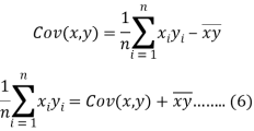
The variance of variable x can be expressed as-


Dividing equation (4) by n, we get-

From the equation (6), (7) and (8)-
Cov (x, y) + 
Multiply (5) by , we get-

Subtracting equation (10) from equation (9), we get-


Since ‘b’ is the slope of the line of regression y on x and the line of regression passes through the point ( ), so that the equation of the line of regression of y on x is-


This is known as regression line of y on x.
Note-
 are the coefficients of regression.
Regression of X on Y | Regression of X on Y |
Assumption: X depends on Y The regression equation is (x- x) = bxy (y- y ) bxy= Regression co-efficient of X onY=Cov (x, y) V (y) | Y depends on X The regression equation is (y- y) = byx (x- x ) byx= Regression co-efficientof YonX=Cov (x,y) V (x) |
Example: Two variables X and Y are given in the dataset below, find the two lines of regression.
x | 65 | 66 | 67 | 67 | 68 | 69 | 70 | 71 |
y | 66 | 68 | 65 | 69 | 74 | 73 | 72 | 70 |
Sol.
The two lines of regression can be expressed as-

And

x | y |  |  | Xy |
65 | 66 | 4225 | 4356 | 4290 |
66 | 68 | 4356 | 4624 | 4488 |
67 | 65 | 4489 | 4225 | 4355 |
67 | 69 | 4489 | 4761 | 4623 |
68 | 74 | 4624 | 5476 | 5032 |
69 | 73 | 4761 | 5329 | 5037 |
70 | 72 | 4900 | 5184 | 5040 |
71 | 70 | 5041 | 4900 | 4970 |
Sum = 543 | 557 | 36885 | 38855 | 37835 |
Now-

And

Standard deviation of x-


Similarly-


Correlation coefficient-


Put these values in regression line equation, we get
Regression line y on x-


Regression line x on y-


Regression line can also be find by the following method-
Example: Find the regression line of y on x for the given dataset.
X | 4.3 | 4.5 | 5.9 | 5.6 | 6.1 | 5.2 | 3.8 | 2.1 |
Y | 12.6 | 12.1 | 11.6 | 11.8 | 11.4 | 11.8 | 13.2 | 14.1 |
Sol.
Let y = a + bx is the line of regression of y on x, where ‘a’ and ‘b’ are given as-


We will make the following table-
x | Y | Xy |  |
4.3 | 12.6 | 54.18 | 18.49 |
4.5 | 12.1 | 54.45 | 20.25 |
5.9 | 11.6 | 68.44 | 34.81 |
5.6 | 11.8 | 66.08 | 31.36 |
6.1 | 11.4 | 69.54 | 37.21 |
5.2 | 11.8 | 61.36 | 27.04 |
3.8 | 13.2 | 50.16 | 14.44 |
2.1 | 14.1 | 29.61 | 4.41 |
Sum = 37.5 | 98.6 | 453.82 | 188.01 |
Using the above equations we get-


On solving these both equations, we get-
a = 15.49 and b = -0.675
So that the regression line is –
y = 15.49 – 0.675x
Example: Show that the geometric mean of the coefficients of regression is the coefficient of correlation.
Sol.
We know that the coefficients of regression are-

Then-

Example: Prove that arithmetic mean of the coefficients of regression is greater than the coefficient of correlation.
Sol.
We know that the coefficients of regression are-

Here we need to prove that- A.M. > r
So that-


Which is true.
Note – Standard error of predictions can be find by the formula given below-

Difference between regression and correlation-
1. Correlation is the linear relationship between two variables while regression is the average relationship between two or more variables.
2. There are only limited applications of correlation as it gives the strength of linear relationship while the regression is to predict the value of the dependent varibale for the given values of independent variables.
3. Correlation does not consider dependent and independent variables while regression consider one dependent variable and other indpendent variables.
Example 3:
The following data give the experience of machine operators and their performance rating given by the number of good parts turned out per 100pieces.
Operator: | 1 | 2 | 3 | 4 | 5 | 6 | 7 | 8 |
Experience: (in year) | 16 | 12 | 18 | 4 | 3 | 10 | 5 | 12 |
Performance: Rating | 87 | 88 | 89 | 68 | 78 | 80 | 75 | 83 |
Obtain the two regression equations and estimate the performance rating of an operator who has put 15 years in service.
Solution: We define the variables,
X: Experience | Y: Performance rating Table of calculations: | |||
X | Y | Xy | X2 | Y2 |
16 12 18 4 3 10 5 12 | 87 88 89 68 78 80 75 83 | 1392 1056 1602 272 232 800 375 996 | 256 144 324 16 9 100 25 144 | 7569 7744 7921 4624 6084 6400 5625 6889 |
 |  |  |  |  |
Now the two regression equations are,
(

Where,
 and
and 
Also,
Co(x,y) 

Co(x,y)=30.75


Now we find,
Regression co-efficient od X on Y


 and
and
Regression xo-efficient of X on Y


Now substituting the values of x , y , bxy and byx in the regression
Equations we get,
(x-10) = 0.67(y-81) -------x on y (i)
(y-81) =1.13(x-10) ------- y on x (ii)
As the two regression equations.
Now to estimate Performance rating (y) when Experience (x) = 15, we use
The regression equation of y on x
(y-81) =1.13(15-10)
y = 81+ 5.65 = 86.65
Hence the estimated performance rating for the operator with 15 years of
Experience is approximately 86.65 i.e. approximately 87
Regression coefficients in terms of correlation coefficient
We can also obtain the regression coefficients bxy and byx from standard deviations,  and correlation coefficient ‘r’ using the formulas.
 and
and 
Also consider,
 i.e.
i.e. 
Hence the correlation coefficient ‘r’ is the geometric mean of the regression coefficients, bxy and byx
Example 4: Find the marks of a student in the Subject of Mathematics who have scored 65 marks in Accountancy Given,
Average marks in Mathematics Accountancy Standard Deviation of marks in Mathematics In accountancy | 70 80 8 10 |
Coefficient of correlation between the marks of Mathematics and marks of Accountancy is 0.64.
Solution: We define the variables,
X: Marks in Mathematics
Y: Marks in Accountancy
Therefore, we have,

Now we want to approximate the marks in Mathematics (x), we obtain the
Regression equation of x on y, which is given by

Substituting the values, we get,

i.e. 
Therefore, when marks in Accountancy (Y) = 65
x- 70 = 0.57(65-80)
x = 70-2.85 = 67.15 i.e. 67 approx.
Substitute the value of a and b in the equation. Regression line of X on Y is 
Example 5:
Find the means values of x,y and r from the two regression equations.
3x+2y-26=0 and sx+y-31=0. Also find sx when sy = 3.
Solution: The two regression equations are,
3x+2y-26=0 -------- (i)
6x+y-31=0 ----------(ii)
Now for x and y we solve the two equations as the simultaneous equations.
On solving (1) and (2), we get-
x = 4 and y = 7.
Now to find ‘r’ we express the equations in the form y=a+bx
So, from eqns (i) and (ii)
 and
and 

since, b1 < b2 (i.e., b1 is smaller in number irrespective of sign + or -)
... Equation (i) is regression of  on
on  and
and 
Hence, eqn (ii) is regression of  on
on  and
and  - 1/6 = - 0.16
Now we find, 
Note: The sign of ‘r’ is same as the sign of regression coefficients
Now to find 6x when 6y = 3, we use the formula,


Hence means 
Example 6: From the following data obtain the two regression equations:
 | 6 | 2 | 10 | 4 | 8 |
 | 9 | 11 | 5 | 8 | 7 |
Solution:
Computation of Regression Equation
X | Y | Xy | x2 | y2 |
6 2 10 4 8 | 9 11 5 8 7 | 54 22 50 32 56 | 36 4 100 16 64 | 81 121 25 64 49 |
 |  |  |  |  |
Regression line of y and X is expressed by the equation of the form 
To determine the values of a and b, the following two normal equations are solved


Substituting the value, we get


Multiplying equation (i) by 6, we get


Deduct equation (iv) from (iii)


Substitute the value of b in equation (i)


Substitute the value of a and b in the equation
Regression line of Y on X is

Regression line X on Y is

The corresponding normal equations are


Substituting the values


Multiply equation (i) by 8


Deduct equation (iv) from (iii)

Substitute the value of b in equation) i)


Substitute the value of a and b in the equation. Regression line of X on Y is 
Example 7 Calculate the regressive coefficients from the data given below:
| Series  | Series  |
|
Average | 25 | 22 |
|
Standard deviation | 4 | 2 | r=0.8 |
Solution: The coefficient of regression of y on x is

The coefficient of regression of y on x is

Example 8: The following scores were worked out from a test in Mathematics and English in an annual examination.
Find both the regression equations. Using these regression estimate finds the value of Y for X=50 and the value of x for Y=30. | ||||||||||||
| ||||||||||||
 
|
Regression Coefficients : X on Y

Y on X

Regression equation: X on Y

Substituting the values
X-75= 0.652 (Y-115)= 0.652Y-74.98
Or 
Where 

Regression equation: Y on X

Y-115= 0.78 (X-75) =0.78 X-58.5
Example 10:
From the following regression equation, find means x , y ,and d ‘r’ 3x-2y-10 = 0, 24x-25y+145 = 0
Solution: The two regression equations are,
3x-2y-10=0(i)
24x-25y+145=0(ii)
Now for x and y we solve the two equations as the simultaneous equations.
Therefore, by (i) x 8 and (ii) x1, we get
24x-16y-80 = 0
24x-25y+145 = 0
9y-225=0y = 25
Putting y = 25 in eqn (i), we get
3x-2(25)-10 = 0
3x – 60=0
X = 20
Hence x= 20 and y= 25.
Now to find ‘r’ we express the equations in the form y=a+bx So, from eqns (i) and (ii)
B1=1.5 b2=0.96
Equation (ii) is regression of y on x and byx = 0.9
Hence eqn (i) is regression of x on y and bxy = 1/1.5 =0.67
Now we find, r = √ bxyXbyxi.e. r=√0.67x0.96= + 0.84
Regression line of least Square Method
It is a mathematical method and with it gives a fitted trend line for the set of data in such a manner that the following two conditions are satisfied.
The sum of the deviations of the actual values of Y and the computed values of Y is zero.
The sum of the squares of the deviations of the actual values and the computed values is least.
This method gives the line which is the line of best fit. This method is applicable to give results either to fit a straight-line trend or a parabolic trend.
The method of least squares as studied in time series analysis is used to find the trend line of best fit to a time series data.
Secular Trend Line
The secular trend line (Y) is defined by the following equation:
Y = a + b X
Where, Y = predicted value of the dependent variable
a = Y-axis intercept i.e. the height of the line above origin (when X = 0, Y = a)
b = slope of the line (the rate of change in Y for a given change in X)
When b is positive the slope is upwards, when b is negative, the slope is downwards
X = independent variable (in this case it is time)
To estimate the constants a and b, the following two equations have to be solved simultaneously:
ΣY = na + b ΣX
ΣXY = aΣX + bΣX2
To simplify the calculations, if the midpoint of the time series is taken as origin, then the negative values in the first half of the series balance out the positive values in the second half so that ΣX = 0. In this case, the above two normal equations will be as follows:
ΣY = na
ΣXY = bΣX2
Q1) Fit the straight line to the following data.
X | 1 | 2 | 3 | 4 | 5 |
Y | 1 | 2 | 3 | 4 | 5 |
A1)
The normal equation are:
Σy = aΣx + nb
And
Σxy = aΣx2 + bΣx
Now,
X | Y |  | XY |
1 | 1 | 1 | 1 |
2 | 2 | 4 | 4 |
3 | 3 | 9 | 9 |
4 | 4 | 16 | 16 |
5 | 5 | 25 | 25 |
 |  |  |  |
15 = 15a + 4b and 55 = 55a + 15b
Solving these two equations,
We get a=1 and b=0,
Therefore the required straight-line equation is y=x.
Regression line Least Square Method
Q2) Fit the straight-line curve to the following data.
X | 75 | 80 | 93 | 65 | 87 | 71 | 98 | 68 | 84 | 77 |
Y | 82 | 78 | 86 | 72 | 91 | 80 | 95 | 72 | 89 | 74 |
A2) First drawing the table,
X | Y |  | XY |
75 | 82 | 5625 | 1 |
80 | 78 | 6400 | 4 |
93 | 86 | 8349 | 9 |
65 | 72 | 4225 | 16 |
87 | 91 | 7569 | 25 |
71 | 80 | 5041 |
|
98 | 95 | 9605 |
|
68 | 72 | 4624 |
|
84 | 89 | 7056 |
|
77 | 74 | 5929 |
|
 |  |  |  |
The normal equation are:
Σy = aΣx + nb
And
Σxy = aΣx2 + bΣx.
Substituting the values, we get,
819 = 798a + 10b
66045 = 64422a + 798b
Solving, we get
a = 0.9288 and b = 7.78155
Therefore, the straight line equation is:
y = 0.9288x + 7.78155.
Key takeaways:
- If the scatter diagram indicates some relationship between two variables
 and
and  , then the dots of the scatter diagram will be concentrated round a curve. This curve is called the curve of regression.
 - Regression line is the best fit line which expresses the average relation between variables.
 are the coefficients of regression.
- The geometric mean of the coefficients of regression is the coefficient of correlation.
- The arithmetic mean of the coefficients of regression is greater than the coefficient of correlation
- Standard error of predictions can be find by the formula given below-

Measures of central tendency
Professor Bowley defines the average as-
“Statistical constants which enable us to comprehend in a single effort the significance of the whole”
An average is a single value which is the best representative for a given data set.
Measures of central tendency show the tendency of some central values around which data tend to cluster.
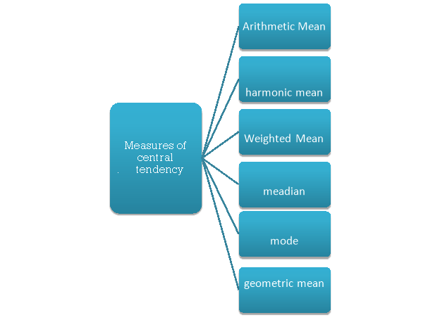
The following are the various measures of central tendency-
1. Arithmetic mean
2. Median
3. Mode
4. Weighted mean
5. Geometric mean
6. Harmonic mean
Arithmetic mean or mean-
Arithmetic mean is a value which is the sum of all observation divided by total number of observations of the given data set.
If there are n numbers in a dataset-  then arithmetic mean will be-

If the numbers along with frequencies are given then mean can be defined as-

Example-1: Find the mean of 26, 15, 29, 36, 35, 30, 14, 21, 25 .
Sol.


Example-2: Find the mean of the following dataset.
x | 20 | 30 | 40 |
f | 5 | 6 | 4 |
Sol.
We have the following table-
x | f | Fx |
20 | 5 | 100 |
30 | 6 | 180 |
40 | 7 | 160 |
| Sum = 15 | Sum = 440 |
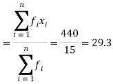
Then Mean will be-

Direct method to find mean-
Example: Find the arithmetic mean of the following dataset-
Class Interval | 0-10 | 10-20 | 20-30 | 30-40 | 40-50 |
Frequency | 3 | 5 | 7 | 9 | 4 |
Sol.
We have the following distribution-
Class interval | Mid value (x) | Frequency (f) | Fx |
0-10 | 05 | 3 | 15 |
10-20 | 15 | 5 | 75 |
20-30 | 25 | 7 | 175 |
30-40 | 35 | 9 | 315 |
40-50 | 45 | 4 | 180 |
|
| Sum = 28 | Sum = 760 |
Mean = 
Short cut method to find mean-
Suppose ‘a’ is assumed mean, and ‘d’ is the deviation of the variate x form a, then-

Example: Find the arithmetic mean of the following dataset.
Class | 0-10 | 10-20 | 20-30 | 30-40 | 40-50 |
Frequency | 7 | 8 | 20 | 10 | 5 |
Sol.
Let the assumed mean (a) = 25,
Class | Mid-value | Frequency | x – 25 = d | Fd |
0-10 | 5 | 7 | -20 | -140 |
10-20 | 15 | 8 | -10 | -80 |
20-30 | 25 | 20 | 0 | 0 |
30-40 | 35 | 10 | 10 | 100 |
40-50 | 45 | 5 | 20 | 100 |
Total |
| 50 |
| -20 |

Step deviation method for mean-

Where
Median-
Median is the mid value of the given data when it is arranged in ascending or descending order.
1. If the total number of values in data set is odd then median is the value of  item.
item.
Note-The data should be arranged in ascending r descending order
2. If the total number of values in data set is even then median is the mean of the  item.
item.
Example: Find the median of the data given below-
7, 8, 9, 3, 4, 10
Sol.
Arrange the data in ascending order-
3, 4, 7, 8, 9, 10
So there total 6 (even) observations, then-


Median for grouped data-

Here,


Example: Find the median of the following dataset-
Class Intervsl | 0 - 10 | 10 - 20 | 20 - 30 | 30 - 40 | 40 - 50 |
Frequency | 3 | 5 | 7 | 9 | 4 |
Sol.
Class interval | Frequency | Cumulative frequency |
0 - 10 | 3 | 3 |
10 – 20 | 5 | 8 |
20 – 30 | 7 | 15 |
30 – 40 | 9 | 24 |
40 – 50 | 4 | 28 |

So that median class is 20-30.
Now putting the values in the formula-


So that the median is 28.57
Mode-
A value in the data which is most frequent is known as mode.
Example: Find the mode of the following data points-

Sol. Here 6 has the highest frequency, so that the mode is 6.
Mode for grouped data-

Here,


Example: Find the mode of the following dataset-
Class Interval | 0 - 10 | 10 - 20 | 20 - 30 | 30 - 40 | 40 - 50 |
Frequency | 3 | 5 | 7 | 9 | 4 |
Sol.
Class interval | Frequency |
0 - 10 | 3 |
10 – 20 | 5 |
20 – 30 | 7 |
30 – 40 | 9 |
40 – 50 | 4 |
Here highest frequency is 9. So that the modal class is 40-50,
Put the values in the given data-


Hence the mode is 42.86
Note-
Mean – Mode = [Mean - Median]
Geometric Mean-
If  are the values of the data, then the geometric mean-

Harmonic mean-
Harmonic mean is the reciprocal of the arithmetic mean-
It can be defined as-

Concept of partition values:
Partition values-
The values divide the distribution into certain number of equal parts are called partition values.
Data should be arranged in ascending order descending order.
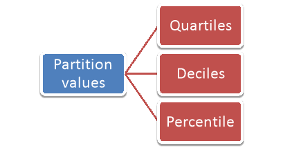
Quartile, deciles and percentile are the partition values.
Note-
- Quartile divides the data into four equal parts.
- Deciles and percentiles divide the distribution into ten and hundred equal parts, respectively
Quartile-
There are three quartiles, i.e. Q1, Q2 and Q3 which divide the total data into four equal parts when it has been orderly arranged. Q1, Q2 and Q3 are termed as first quartile, second quartile and third quartile or lower quartile, middle quartile and upper quartile, respectively. The first quartile, Q1, separates the first one-fourth of the data from the upper three fourths and is equal to the 25th percentile. The second quartile, Q2, divides the data into two equal parts (like median) and is equal to the 50th percentile. The third quartile, Q3, separates the first three-quarters of the data from the last quarter and is equal to 75th percentile.
For ungrouped data, we find the quartiles as follows-


For grouped data, we find the quartiles as follows-
i’th quartile can be find as-

l = lower class limit of i'th quartile class,
h = width of the ith quartile class,
N = total frequency,
C = cumulative frequency of pre ith quartile class, and
f = frequencies of ith quartile class.
Deciles
Deciles divide whole distribution in to ten equal parts. There are nine deciles.
For ungrouped data, we find the deciles as follows-

For grouped data, we find the deciles as follows-
i’th decile can be find as-

Percentile-
Percentiles divide whole distribution in to 100 equal parts. There are ninety nine percentiles.
For ungrouped data, we find the percentile as follows-

For grouped data, we find the percentile as follows-
i’th percentile can be find as-

Example: Calculate the first and third quartile of the following data-
Class interval | f |
0-10 | 3 |
10-20 | 5 |
20-30 | 7 |
30-40 | 9 |
40-50 | 4 |
Sol.
Class interval | f | CF |
0-10 | 3 | 3 |
10-20 | 5 | 8 |
20-30 | 7 | 15 |
30-40 | 9 | 24 |
40-50 | 4 | 28 |
| N = 28 |
|
Here N/4 = 28/4 = 7
The 7th observation falls in the class 10-20. So, this is the first quartile class. 3N/4 = 21th observation falls in class 30-40, so it is the third quartile class.
For first quartile l = 10, f = 5, C = 3, N = 28
We know that-


For third quartile l = 30, f = 9, C = 15

Measures of dispersions:
As the name suggests, the measure of dispersion shows the scatterings of the data. It tells the variation of the data from one another and gives a clear idea about the distribution of the data. The measure of dispersion shows the homogeneity or the heterogeneity of the distribution of the observations.
According to Spiegel, the degree to which numerical data tend to spread about an average value is called the variation or dispersion of data.
Classification of Measures of Dispersion
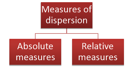
There are two basic kinds of a measure of dispersion-
- Absolute measures
- Relative measures
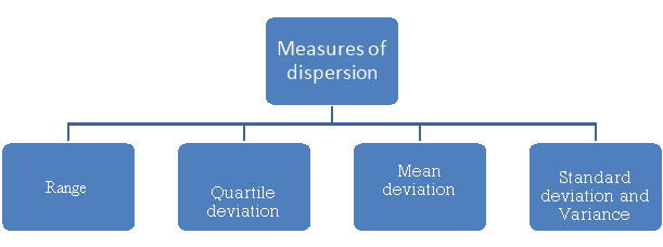
Following are the different types of measures of dispersion-
According to Spiegel-
“The degree to which numerical data tend to spread about an average value is called the variation or dispersion of data”
The different measures of dispersion are-
1. Range
2. Quartile deviation
3. Mean deviation
4. Standard deviation
5. Variance
Significance of measures of dispersion-
Measures of variation are pointed out as to how far an average is representative of the entire data. When variation is less, the average closely represents the individual values of the data and when variation is large; the average may not closely represent all the units and be quite unreliable.
Another purpose of measuring variation is to determine the nature and causes of variations in order to control the variation itself. Measurements of dispersion are helpful to control the causes of variation.
Many powerful statistical tools in statistics such as correlation analysis, the testing of hypothesis, the analysis of variance, techniques of quality control, etc. are based on different measures of dispersion.
Range
Range is the simplest measure of dispersion. Range is the difference between the maximum value of the variable and the minimum value of the variable in the distribution.

Example: Find the range of the distribution 4, 22, 14, 12, 16, 8, 13, 17, 21, 6, 5, 26.
Sol.
For the given distribution, the maximum value is 26 and the minimum value is 4, so that the range of the distribution is –

Example- Find the range of the data- 8, 5, 6, 4, 7, 10, 12, 15, 25, 30
Sol. Here the maximum value is 30 and the minimum value is 4 so that the range is-
30 – 4 = 26
Coefficient of range-
The coefficient of range can be calculated as follows-
Coefficient of Range = 
Advantages of range-
- It is very simple to calculate
- It has useful applications in areas like order statistics and statistical quality control.
Disadvantages of range-
- It utilizes only the maximum and the minimum values of variable in the series and gives no importance to other observations
- It is affected by fluctuations of sampling
- If a single value lower than the minimum or higher than the maximum is added or if the maximum or minimum value is deleted range is seriously affected
Quartile Deviation
The quartiles divide a data set into quarters. The first quartile, (Q1) is the middle number between the smallest number and the median of the data. The second quartile, (Q2) is the median of the data set. The third quartile, (Q3) is the middle number between the median and the largest number.
Quartile deviation or semi-inter-quartile deviation is

Relative measure of Q.D. Known as Coefficient of Q.D. And is defined as

Example: Find the quartile deviation of the following data.
Class interval | 0-10 | 10-20 | 20-30 | 30-40 | 40-50 |
Frequency | 3 | 5 | 7 | 9 | 4 |
Sol.
We have N/4 = 28/4 = 7 and 7th observation falls in the class 10-20.
This is the first quartile class. Similarly, 3N/4 = 21 and 21st observation falls in the interval 30-40. This is the third quartile class.
Class interval | f | CF |
0-10 | 3 | 3 |
10-20 | 5 | 8 |
20-30 | 7 | 15 |
30-40 | 9 | 24 |
40-50 | 4 | 28 |
| N = 28 |
|
By using the formula of quartile deviation, we will find  -
-


Therefore-
Q = ½ × (Q3 – Q1) = (36.67 – 18) / 2 = 9.335
Example: Find the quartile deviation of the following data-
Class | 0-5 | 5-10 | 10-15 | 15-20 | 20-25 | 25-30 | 30-35 | 35-40 |
Frequency | 6 | 8 | 12 | 24 | 36 | 32 | 24 | 8 |
Sol.
We will construct the cumulative frequency table-
Class interval | f | CF |
0-5 | 6 | 6 |
5-10 | 8 | 14 |
10-15 | 12 | 26 |
15-20 | 24 | 50 |
20-25 | 36 | 86 |
25-30 | 32 | 118 |
30-35 | 24 | 142 |
35-40 | 8 | 150 |
| N = 150 |
|
We know that-

So that

And

Therefore-
Q = ½ × (Q3 – Q1) = (30.52 – 17.40) / 2 = 6.56
Key takeaways-
- The measure of dispersion shows the homogeneity or the heterogeneity of the distribution of the observations.
- The degree to which numerical data tend to spread about an average value is called the variation or dispersion of data.

Mean Deviation
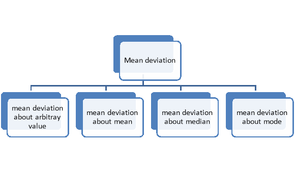
Mean deviation is the average of the sum of the absolute values of deviation from any arbitrary value viz. Mean, median, mode, etc.
The deviation of an observation xi from the assumed mean A is defined as (xi – A).
Therefore,
The mean deviation can be defined as-

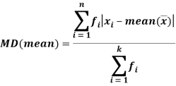
Mean deviation from mean is defined as-

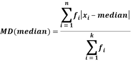
Mean deviation from median is defined as-

For frequency distribution-
Example: Find the mean deviation from mean of the following data-
x | 1 | 2 | 3 | 4 | 5 | 6 | 7 |
f | 3 | 5 | 8 | 12 | 10 | 7 | 5 |
Sol.
x | F | Fx | |x-  | f|x-  |
1 | 3 | 3 | 3.24 | 9.72 |
2 | 5 | 10 | 2.24 | 11.20 |
3 | 8 | 24 | 1.24 | 9.92 |
4 | 12 | 48 | 0.24 | 2.88 |
5 | 10 | 50 | 0.76 | 7.60 |
6 | 7 | 42 | 1.76 | 12.32 |
7 | 5 | 35 | 2.76 | 13.80 |
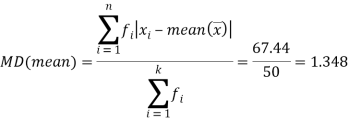
Total | 50 | 212 | 12.24 | 67.44 |

We know that-
Example: The students of statistics got the marks as below-
16, 24, 13, 18, 15, 10, 23
Find the mean deviation from mean.
Sol.
X | x-17 | |x-  |
16 | -1 | 1 |
24 | 7 | 7 |
13 | -4 | 4 |
18 | 1 | 1 |
15 | -2 | 2 |
10 | -7 | 7 |
23 | 6 | 6 |
Sum = 119 |
| 28 |
Then

Hence

Example 11. Find the mean deviation of the following frequency distribution
Class | 0-6 | 6-12 | 12-18 | 18-24 | 24-30 |
Frequency | 8 | 10 | 12 | 9 | 5 |
Solution. Let a = 15
Class | Mid-value x | Frequency f | d = x-a | Fd | |x-14| | f|x-14| |
0-6 | 3 | 8 | -12 | -96 | 11 | 88 |
6-12 | 9 | 10 | -6 | -60 | 5 | 50 |
12-18 | 15 | 12 | 0 | 0 | 1 | 12 |
18-24 | 21 | 9 | +6 | 54 | 7 | 63 |
24-30 | 27 | 5 | +12 | 60 | 13 | 65 |
Total |
| 44 |
| -42 |
| 278 |

Then mean deviation from mean-

Standard deviation, variance & combined Variance
Variance-
Variance is the average of the square of deviations of the values taken from mean. Taking a square of the deviation is a better technique to get rid of negative deviations.
Variance is given as-

And for a frequency distribution, the formula is

Variance of the combined series-
If σ1, σ2 are two standard deviations of two series of sizes n1 and n2 with means ȳ1 and ȳ2. The variance of the two series of sizes n1 + n2 is:
σ 2 = (1/ n1 + n2) ÷ [n1 (σ1 2 + d1 2) + n2 (σ2 2 + d2 2)]
Where, d1 = ȳ 1 −ȳ , d2 = ȳ 2 −ȳ , and ȳ = (n1 ȳ 1 + n2 ȳ 2) ÷ ( n1 + n2).
Coefficient of variation
Coefficient of variation can be calculated as-

Note- The lower value of C.V, the more constancy of data
Example- If student A has a mean 50 with SD 10.Another student B has a mean of 30 with SD = 3.
Which one is the best performer?
Sol. We calculate C.V.-


And

Here B has a lower C.V. So that student B is the best performer.
Example: Calculate coefficient variation for the following frequency distribution.
Wages in Rupees earned per day | 0-10 | 10-20 | 20-30 | 30-40 | 40-50 | 50-60 |
No. Of Labourers | 5 | 9 | 15 | 12 | 10 | 3 |
Solution:
We already calculated

Now,
A.M 

A.M 
 Coefficient of Variation


Example: Suppose batsman A has mean 50 with SD 10. Batsman B has mean 30 with SD 3. What do you infer about their performance?
Sol.
A has higher mean than B. This means A is a better run maker.
However, B has lower CV (3/30 = 0.1) than A (10/50 = 0.2) and is consequently more consistent.
Note-
It is a relative measure of variability. If we are comparing the two data series, the data series having smaller CV will be more consistent.
Standard deviation-
It is defined as the positive square root of the arithmetic mean of the square of the deviation of the given values from their arithmetic mean. It is denoted by the symbol  .
.

Where  is A.M of the distribution
  . We have more formulae to calculate the standard deviation.


 ….
…. 
In frequency distribution from, we put  where H is generally taken as width of class interval


Shortcut formula to calculate standard deviation-

The square of the standard deviation is called known as a variance.

Example: Find the Variance and Standard Deviation of the Following Numbers: 1, 3, 5, 5, 6, 7, 9, 10.
Sol.
The mean = 46/ 8 = 5.75
Step 1: (1 – 5.75), (3 – 5.75), (5 – 5.75), (5 – 5.75), (6 – 5.75), (7 – 5.75), (9 – 5.75), (10 – 5.75)
= -4.75, -2.75, -0.75, -0.75, 0.25, 1.25, 3.25, 4.25
Step 2: Squaring the above values we get, 22.563, 7.563, 0.563, 0.563, 0.063, 1.563, 10.563, 18.063
Step 3: 22.563 + 7.563 + 0.563 + 0.563 + 0.063 + 1.563 + 10.563 + 18.063
= 61.504
Step 4: n = 8, therefore variance (σ2) = 61.504/ 8 = 7.69
Now, Standard deviation (σ) = 2.77
Example: Suppose a series of 100 data points has mean 50 and variance 20. Another series of 200 data points has mean 80 and variance 40. What is the combined variance of the given series?
Sol.
The mean of the combined series-

Therefore, d1= 50 – 70 = –20 and d2 = 80 – 70 =10
Variance of the combined series


Example: Find the standard deviation for the following numbers:
10, 27, 40, 60, 33, 30, 10
Sol.
First we prepare the following distribution table
X |  |
10 | 100 |
27 | 729 |
40 | 1600 |
60 | 3600 |
33 | 1089 |
30 | 900 |
10 | 100 |
Sum = 210 | 8118 |
Then-
Mean = 210 / 7 = 30
And standard deviation-


Example-1: Compute the variance and standard deviation.
Class | Frequency |
0-10 | 3 |
10-20 | 5 |
20-30 | 7 |
30-40 | 9 |
40-50 | 4 |
Sol.
Class | Mid-value (x) | Frequency (f) |  |
0-10 | 5 | 3 | 1470.924 |
10-20 | 15 | 5 | 737.250 |
20-30 | 25 | 7 | 32.1441 |
30-40 | 35 | 9 | 555.606 |
40-50 | 45 | 4 | 1275.504 |
Sum |
|  | 4071.428 |

Then standard deviation,

Example-2: Calculate the standard deviation of the following frequency distribution-
Weight | 60 – 62 | 63 – 65 | 66 – 68 | 69 – 71 | 72 – 74 |
Item | 5 | 18 | 42 | 27 | 8 |
Sol.
Weight | Item (f) | X | d = x – 67 | f.d |  |
60 – 62 | 5 | 61 | -6 | -30 | 180 |
63 – 65 | 18 | 64 | -3 | -54 | 162 |
66 – 68 | 42 | 67 | 0 | 0 | 0 |
69 – 71 | 27 | 70 | 3 | 81 | 243 |
72 – 74 | 8 | 73 | 6 | 48 | 288 |
Total |
100 |
|
|
45 |
873 |


Example: Calculate S.D for the following distribution.
Wages in rupees earned per day | 0-10 | 10-20 | 20-30 | 30-40 | 40-50 | 50-60 |
No. Of Labourers | 5 | 9 | 15 | 12 | 10 | 3 |
Solution:
Wages earned C.I | Mid value  | Frequency |  |  |  |
52 | 5 | 5 | -2 | -10 | 20 |
153 | 15 | 9 | -1 | -9 | 9 |
25 | 25 | 15 | 0 | 0 | 0 |
35 | 35 | 12 | 1 | 12 | 12 |
45 | 45 | 10 | 2 | 20 | 40 |
55 | 55 | 3 | 3 | 9 | 27 |
Total | - |  |  |  |  |
Using formula,


Key takeaways-
- The measure of dispersion shows the homogeneity or the heterogeneity of the distribution of the observations.
- The degree to which numerical data tend to spread about an average value is called the variation or dispersion of data.


- Range = Max. Value – Min. Value
- Coefficient of Range =


The word skewness means lack of symmetry. Lack of symmetry is called skewness for a frequency distribution. If the distribution is not symmetric, the frequencies will not be uniformly distributed about the centre of the distribution.
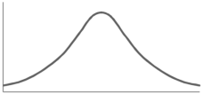
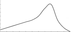
The examples of symmetric curve, positively skewed and negatively skewed curves are given as follows-
1. Symmetric curve-
2. Positively skewed-
3. Negatively skewed-
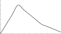
Skewness denotes the opposite of symmetry. In a symmetrical series, the mode, the median, and the arithmetic average are identical.
Measures of skewness:
There are two types of measures of skewness-
- Absolute measures of skewness
- Relative measures of skewness
Absolute Measures of Skewness:
Following are the absolute measures of skewness:
1. Skewness = Mean – Median
2. Skewness = Mean – Mode
3. Skewness = (Q3 - Q2) - (Q2 - Q1)
Relative Measures of Skewness:
 coefficient of skewness:
Karl Pearson defined the following  and
and  coefficients of skewness,
Based upon the second and third central moments:

It is used as measure of skewness. For a symmetrical distribution,  shall be zero.
  as a measure of skewness does not tell about the direction of skewness, i.e. positive or negative. Because
  being the sum of cubes of the deviations from mean may be positive or negative but
  is always positive. Also,
  being the variance always positive. Hence,
  would be always positive. This drawback is removed if we calculate Karl Pearson’s Gamma coefficient
  which is the square root of
  i. e.
i. e.

Then the sign of skewness would depend upon the value of  whether it is positive or negative. It is advisable to use
  as measure of skewness.
Karl Pearson’s coefficient of skewness-
Then formula is as follows-

The value of this coefficient would be zero in a symmetrical distribution. If mean is greater than mode, coefficient of skewness would be positive otherwise negative. The value of the Karl Pearson’s coefficient of skewness usually lies between  1 for moderately skewed distubution.
If mode is not well defined, we can use the formula

By using the relationship
Mode = (3 Median – 2 Mean)
Bowleys’s Coefficient of Skewness:
This formula is based on quartiles:

The value of this coefficient would be zero if it is a symmetrical distribution. If the value is greater than zero, it is positively skewed and if the value is less than zero it is negatively skewed distribution. It will take value between +1 and -1.
Kelly’s Coefficient of Skewness:
The coefficient of skewness given by Kelly is based on percentiles and deciles. The formula for calculating the coefficient of skewness is given by

Difference between Variance and Skewness:
1. Variance is the amount of variability while skewness gives the direction of variability.
2. In business and economic series, measures of variation have greater practical application than measures of skewness. However, in medical and life science field measures of skewness have greater practical applications than the variance.
Example: Calculate the coefficient of skewness from the following data:
Weight (lbs) | 70-80 | 80-90 | 90-100 | 100-110 | 110-120 | 120-130 | 130-140 | 140=150 |
No. Of persons | 12 | 18 | 35 | 42 | 50 | 45 | 20 | 8 |
Sol:
Here total frequency 
The cumulative frequency table is
Weight (lbs) | 70-80 | 80-90 | 90-100 | 100-110 | 110-120 | 120-130 | 130-140 | 140=150 |
Frequency | 12 | 18 | 35 | 42 | 50 | 45 | 20 | 8 |
Cumulative Frequency | 12 | 30 | 65 | 107 | 157 | 202 | 222 | 230 |
Now, N/2 =230/2= 115th item which lies in 110 – 120 group.
Median or 
Also,  is 57.5th or 58th item which lies in 90-100 group.

Similarly 3N/4 = 172.5 i.e.  is 173rd item which lies in 120-130 group.

Hence quartile coefficient of skewness = 

Example: If coefficient of skewness is 0.64. Standard deviation is 13 and mean is 59.2, then find the mode and median.
Sol.
We know that-

So that-


And we also know that-


Example: Calculate the Karl Pearson’s coefficient of skewness of marks obtained by 150 students.
Marks | 0 - 10 | 10 - 20 | 20 - 30 | 30 - 40 | 40 - 50 | 50 – 60 | 60 – 70 | 70 – 80 |
No. Of Students | 10 | 40 | 20 | 0 | 10 | 40 | 16 | 14 |
Sol. Mode is not well defined so that first we calculate mean and median-
Class | f | x | CF |  | Fd |  |
0-10 | 10 | 5 | 10 | -3 | -30 | 90 |
10-20 | 40 | 15 | 50 | -2 | -80 | 160 |
20-30 | 20 | 25 | 70 | -1 | -20 | 20 |
30-40 | 0 | 35 | 70 | 0 | 0 | 0 |
40-50 | 10 | 45 | 80 | 1 | 10 | 10 |
50-60 | 40 | 55 | 120 | 2 | 80 | 160 |
60-70 | 16 | 65 | 136 | 3 | 48 | 144 |
70-80 | 14 | 75 | 150 | 4 | 56 | 244 |
Now,


And

Standard deviation-

Then-


Example: For a distribution Karl Pearson’s coefficient of skewness is 0.64, standard deviation is 13 and mean is 59.2 Find mode and median.
Sol:
It is given that:
Coeff. Of skewness = 0.64, σ = 13 and Mean = 59.2
Therefore by using formula


Mode = 59.20 – 8.32 = 50.88
Mode = 3 Median – 2 Mean
50.88 = 3 Median - 2 (59.2)

Notes-
1. If the value of mean, median and mode are same in any distribution, then the skewness does not exist in that distribution. Larger the difference in these values, larger the skewness;
2. If sum of the frequencies are equal on the both sides of mode then skewness does not exist.
3. If the distance of first quartile and third quartile are same from the median then a skewness does not exist.
4. If the sums of positive and negative deviations obtained from mean, median or mode are equal then there is no asymmetry
5. If a graph of a data become a normal curve and when it is folded at middle and one part overlap fully on the other one then there is no asymmetry.
Key takeaways:
- The word skewness means lack of symmetry. Lack of symmetry is called skewness for a frequency distribution.
- Skewness denotes the opposite of symmetry. In a symmetrical series, the mode, the median, and the arithmetic average are identical.
- Skewness = Mean – Median


- Karl Pearson’s coefficient of skewness


7. Mode = (3 Median – 2 Mean)
8. Bowleys’s Coefficient of Skewness:

9. Kelly’s Coefficient of Skewness:

References:
- E. Kreyszig, “Advanced Engineering Mathematics”, John Wiley & Sons, 2006.
- P. G. Hoel, S. C. Port And C. J. Stone, “Introduction To Probability Theory”, Universal Book Stall, 2003.
- S. Ross, “A First Course in Probability”, Pearson Education India, 2002.
- W. Feller, “An Introduction To Probability Theory and Its Applications”, Vol. 1, Wiley, 1968.
- N.P. Bali and M. Goyal, “A Text Book of Engineering Mathematics”, Laxmi Publications, 2010.
- B.S. Grewal, “Higher Engineering Mathematics”, Khanna Publishers, 2000.