Unit - 1
Introduction to algorithms
A data structure is a collection of data pieces that provides an efficient method for storing and organizing data in a computer so that it may be used effectively. Arrays, Linked Lists, Stacks, Queues, and other Data Structures are examples. Data Structures are employed in practically every element of computer science, including operating systems, compiler design, artificial intelligence, graphics, and many more applications.
Data Structures are an important aspect of many computer science algorithms because they allow programmers to efficiently handle data. It is critical to improving the performance of a software or program because the software's primary duty is to save and retrieve user data as quickly as feasible.
The building blocks of every program or software are data structures. The most challenging challenge for a programmer is deciding on a suitable data structure for a program. When it comes to data structures, the following terminology is utilized.
Data: The data on a student can be defined as an elementary value or a set of values, for example, the student's name and id.
Group items: Group items are data items that include subordinate data items, such as a student's name, which can have both a first and a last name.
Record: A record can be characterized as a collection of several data objects. For example, if we consider the student entity, the name, address, course, and grades can all be gathered together to constitute the student's record.
File: A file is a collection of various records of one type of entity; for example, if there are 60 employees in the class, the relevant file will contain 20 records, each containing information about each employee.
Attribute and Entity: A class of objects is represented by an entity. It has a number of characteristics. Each attribute represents an entity's specific property.
Need of Data Structures
As applications are getting complexed and amount of data is increasing day by day, there may arise the following problems:
Processor speed: To handle very large amount of data, high speed processing is required, but as the data is growing day by day to the billions of files per entity, processor may fail to deal with that much amount of data.
Data Search: Consider an inventory size of 106 items in a store, If our application needs to search for a particular item, it needs to traverse 106 items every time, results in slowing down the search process.
Multiple requests: If thousands of users are searching the data simultaneously on a web server, then there are the chances that a very large server can be failed during that process
In order to solve the above problems, data structures are used. Data is organized to form a data structure in such a way that all items are not required to be searched and required data can be searched instantly.
Advantages of Data Structures
Efficiency: Efficiency of a program depends upon the choice of data structures. For example: suppose, we have some data and we need to perform the search for a particular record. In that case, if we organize our data in an array, we will have to search sequentially element by element. Hence, using array may not be very efficient here. There are better data structures which can make the search process efficient like ordered array, binary search tree or hash tables.
Reusability: Data structures are reusable, i.e. once we have implemented a particular data structure, we can use it at any other place. Implementation of data structures can be compiled into libraries which can be used by different clients.
Abstraction: Data structure is specified by the ADT which provides a level of abstraction. The client program uses the data structure through interface only, without getting into the implementation details.
Types of data structure
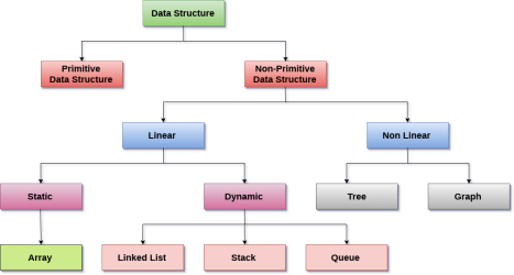
Linear data structure
In Data structure is linear. The processing of data items can be done in a linear fashion, that is, one by one. A linear structure is a data structure that can hold a large number of objects. The things can be added in a variety of ways, but once added, they maintain a constant relationship with their neighbors. For example, a collection of numbers, a collection of strings, and so on.
Once an item is added, it remains in its current location in relation to the things that came before and after it.
Example
● Array
● Linked list
● Stack
● Queue
Array
An array is a collection of data elements of similar types, each of which is referred to as an element of the array. The element's data type can be any valid data type, such as char, int, float, or double.
The array's elements all have the same variable name, but each one has a different subscript number. One-dimensional, two-dimensional, or multidimensional arrays are all possible.
The age array's individual elements are as follows:
Age[0], age[1], age[2], age[3],......... Age[98], age[99].
Linked list
A linked list is a type of linear data structure that is used to keep track of a list in memory. It's a collection of nodes that are stored in non-contiguous memory regions. Each node in the list has a pointer to the node next to it.
Stack
A stack is a linear list with only one end, termed the top, where insertions and deletions are permitted.
A stack is an abstract data type (ADT) that can be used in a variety of programming languages. It's called a stack because it behaves like a real-life stack, such as a stack of plates or a deck of cards.
Queue
A queue is a linear list in which elements can only be added at one end, called the back end, and deleted at the other end, called the front end.
It's a data structure that's similar to a stack. Because the queue is open on both ends, the data items are stored using the First-In-First-Out (FIFO) approach.
Non - linear data structure
The processing of data items in a non-linear data structure is not linear.
Example
● Tree
● Graph
Tree
Trees are multilevel data structures containing nodes that have a hierarchical relationship between them. Leaf nodes are at the bottom of the hierarchical tree, whereas root nodes are at the top. Each node has pointers that point to other nodes.
The parent-child relationship between the nodes is the basis of the tree data structure. Except for the leaf nodes, each node in the tree can have several children, although each node can only have one parent, with the exception of the root node.
Graph
Graphs can be defined as a graphical depiction of a collection of elements (represented by vertices) connected by edges. A graph differs from a tree in the sense that a graph can have a cycle, but a tree cannot.
Operations
- Traversing
The set of data elements is present in every data structure. Traversing a data structure is going through each element in order to perform a certain action, such as searching or sorting.
For example, if we need to discover the average of a student's grades in six different topics, we must first traverse the entire array of grades and calculate the total amount, then divide that sum by the number of subjects, which in this case is six, to find the average.
2. Insertion
The process of adding elements to the data structure at any position is known as insertion.
We can only introduce n-1 data elements into a data structure if its size is n.
3. Deletion
Deletion is the process of eliminating an element from a data structure. We can remove an element from the data structure at any point in the data structure.
Underflow occurs when we try to delete an element from an empty data structure.
4. Searching
Searching is the process of discovering an element's location within a data structure. There are two types of search algorithms: Linear Search and Binary Search.
5. Sorting
Sorting is the process of putting the data structure in a specified order. Sorting can be done using a variety of algorithms, such as insertion sort, selection sort, bubble sort, and so on.
6. Merging
Merging occurs when two lists, List A and List B, of size M and N, respectively, containing comparable types of elements are combined to form a third list, List C, of size (M+N).
Key takeaway
A data structure is a collection of data pieces that provides an efficient method for storing and organizing data in a computer so that it may be used effectively.
Arrays, Linked Lists, Stacks, Queues, and other Data Structures are examples.
Data Structures are an important aspect of many computer science algorithms because they allow programmers to efficiently handle data.
If we consider X to be an algorithm and N to be the size of the input data, the time and space implemented by Algorithm X are the two key criteria that determine X's efficiency.
Time Factor - The time is determined or assessed by measuring the number of critical operations in the sorting algorithm, such as comparisons.
Space Factor - The space is estimated or measured by counting the algorithm's maximum memory requirements.
With respect to N as the size of input data, the complexity of an algorithm f(N) provides the running time and/or storage space required by the method.
Space complexity
The amount of memory space required by an algorithm during its life cycle is referred to as its space complexity.
The sum of the following two components represents the amount of space required by an algorithm.
A fixed component is a space needed to hold specific data and variables (such as simple variables and constants, program size, and so on) that are independent of the problem's size.
A variable part is a space that variables require and whose size is entirely dependent on the problem's magnitude. Recursion stack space, dynamic memory allocation, and so forth.
Complexity of space Any algorithm p's S(p) is S(p) = A + Sp (I) Where A is the fixed component of the algorithm and S(I) is the variable part of the algorithm that is dependent on the instance characteristic I. Here's a basic example to help you understand the concept.
Algorithm
SUM(P, Q)
Step 1 - START
Step 2 - R ← P + Q + 10
Step 3 - Stop
There are three variables here: P, Q, and R, as well as one constant. As a result, S(p) = 1+3. Now, the amount of space available is determined by the data types of specified constant types and variables, and it is multiplied accordingly.
Time complexity
The time complexity of an algorithm is a representation of how long it takes for the algorithm to complete its execution. Time requirements can be expressed or specified as a numerical function t(N), where N is the number of steps and t(N) is the time taken by each step.
When adding two n-bit numbers, for example, N steps are taken. As a result, the total processing time is t(N) = c*n, where c represents the time spent adding two bits. We can see that as the input size grows, t(N) climbs linearly.
Let's understand the time complexity through an example.
- Sum=0;
- // Suppose we have to calculate the sum of n numbers.
- For i=1 to n
- Sum=sum+i;
- // when the loop ends then sum holds the sum of the n numbers
- Return sum;
In the above code, the time complexity of the loop statement will be at least n, and if the value of n increases, then the time complexity also increases. While the complexity of the code, i.e., return sum will be constant as its value is not dependent on the value of n and will provide the result in one step only. We generally consider the worst-time complexity as it is the maximum time taken for any given input size.
Key takeaway
The time complexity of an algorithm is the amount of time required to complete the execution.
An algorithm's space complexity is the amount of space required to solve a problem and produce an output.
To express the running time complexity of algorithm three asymptotic notations are available. Asymptotic notations are also called as asymptotic bounds. Notations are used to relate the growth of complex functions with the simple function. Asymptotic notations have a domain of natural numbers.
Big Oh (O) Notation:
- It is the formal way to express the time complexity.
- It is used to define the upper bound of an algorithm’s running time.
- It shows the worst-case time complexity or largest amount of time taken by the algorithm to perform a certain task.
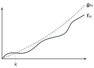
Fig: Big Oh notation
Here, f (n) <= g (n) …………….(eq1)
Where n>= k, C>0 and k>=1
If any algorithm satisfies the eq1 condition then it becomes f (n)= O (g (n))
Consider the following example

In the above example g(n) is ‘’n’ and f(n) is ‘2n+1’ and value of constant is 3. The point where c*g(n) and f(n) intersect is ‘’n0’. Beyond ‘n0’ c*g(n) is always greater than f(n) for constant ‘3’. We can write the conclusion as follows
f(n)=O g(n) for constant ‘c’ =3 and ‘n0’=1
Such that f(n)<=c*g(n) for all n>n0
Big Omega (ῼ) Notation
- It is the formal way to express the time complexity.
- It is used to define the lower bound of an algorithm’s running time.
- It shows the best-case time complexity or best of time taken by the algorithm to perform a certain task.
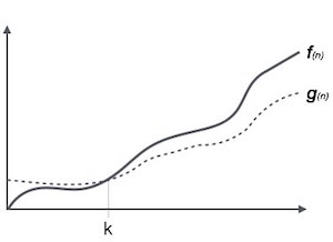
Fig: Big omega notation
Here, f (n) >= g (n)
Where n>=k and c>0, k>=1
If any algorithm satisfies the eq1 condition then it becomes f (n)= ῼ (g (n))
Consider the following example
In the above example g(n) is ‘2n’ and f(n) is ‘2n-2’ and value of constant is 0.5. The point where c*g(n) and f(n) intersect is ‘’n0’. Beyond ‘n0’ c*g(n) is always smaller than f(n) for constant ‘0.5’. We can write the conclusion as follows
f(n) = Ω g(n) for constant ‘c’ =0.5 and ‘n0’=2
Such that c*g(n)<= f(n) for all n>n0

Theta (Θ) Notation
- It is the formal way to express the time complexity.
- It is used to define the lower as well as upper bound of an algorithm’s running time.
- It shows the average case time complexity or average of time taken by the algorithm to perform a certain task.
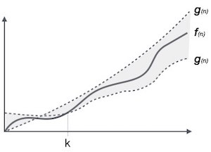
Fig: Theta notation
Let C1 g(n) be upper bound and C2 g(n) be lower bound.
C1 g(n)<= f (n)<=C2 g(n)
Where C1, C2>0 and n>=k
Consider the following example

In the above example g(n) is ‘2n’ and f(n) is ‘3n-2’ and value of constant c1 is 0.5 and c2 is 2. The point where c*g(n) and f(n) intersect is ‘’n0’. Beyond ‘n0’ c1*g(n) is always smaller than f(n) for constant ‘0.5’ and c2*g(n) is always greater than f(n) for constant ‘2’. We can write the conclusion as follows
f(n)=Ω g(n) for constant ‘c1’ =0.5, ‘c2’ = 2 and ‘n0’=2
Such that c1*g(n)<= f(n)<=c2*g(n) for all n>n0
Key takeaway
Big Oh is used to define the upper bound of an algorithm’s running time.
Big Omega is used to define the lower bound of an algorithm’s running time.
Theta is used to define the lower as well as upper bound of an algorithm’s running time.
We all know that as the input size (n) grows, the running time of an algorithm grows (or stays constant in the case of constant running time). Even if the input has the same size, the running duration differs between distinct instances of the input. In this situation, we examine the best, average, and worst-case scenarios. The best case running time is the shortest, the worst case running time is the longest, and the average case running time is the time required to execute the algorithm on average. All of these principles will be explained using two examples: I linear search and (ii) insertion sort.
Best case
Consider the case of Linear Search, in which we look for a certain item in an array. We return the relevant index if the item is in the array; else, we return -1. The linear search code is provided below.
Int search(int a, int n, int item) {
Int i;
For (i = 0; i < n; i++) {
If (a[i] == item) {
Return a[i]
}
}
Return -1
}
Variable an is an array, n is the array's size, and item is the array item we're looking for. It will return the index immediately if the item we're seeking for is in the very first position of the array. The for loop is just executed once. In this scenario, the complexity will be O. (1). This is referred to be the best case scenario.
Average case
On occasion, we perform an average case analysis on algorithms. The average case is nearly as severe as the worst scenario most of the time. When attempting to insert a new item into its proper location using insertion sort, we compare the new item to half of the sorted items on average. The complexity remains on the order of n2, which corresponds to the worst-case running time.
Analyzing an algorithm's average behavior is usually more difficult than analyzing its worst-case behavior. This is due to the fact that it is not always clear what defines a "average" input for a given situation. As a result, a useful examination of an algorithm's average behavior necessitates previous knowledge of the distribution of input instances, which is an impossible condition. As a result, we frequently make the assumption that all inputs of a given size are equally likely and do the probabilistic analysis for the average case.
Worst case
In real life, we almost always perform a worst-case analysis on an algorithm. The longest running time for any input of size n is called the worst case running time.
The worst case scenario in a linear search is when the item we're looking for is at the last place of the array or isn't in the array at all. We must run through all n elements in the array in both circumstances. As a result, the worst-case runtime is O. (n). In the case of linear search, worst-case performance is more essential than best-case performance for the following reasons.
● Rarely is the object we're looking for in the first position. If there are 1000 entries in the array, start at 1 and work your way up. There is a 0.001% probability that the item will be in the first place if we search it at random from 1 to 1000.
● Typically, the item isn't in the array (or database in general). In that situation, the worst-case running time is used.
Similarly, when items are reverse sorted in insertion sort, the worst case scenario occurs. In the worst scenario, the number of comparisons will be on the order of n2, and hence the running time will be O (n2).
Knowing an algorithm's worst-case performance ensures that the algorithm will never take any longer than it does today.
Key takeaway
The best case running time is the shortest, the worst case running time is the longest, and the average case running time is the time required to execute the algorithm on average.
In the selection sort, the smallest value among the array's unsorted items is chosen in each pass and inserted into the proper spot.
To begin, locate the array's smallest element and set it in the first position. Then locate the array's second smallest element and set it in the second spot. The procedure is repeated till the sorted array is obtained.
The n-1 pass of the selection sort algorithm is used to sort the array of n entries.
● The smallest element of the array, as well as its index pos, must be identified in the first run. Swap A[0] and A[pos] after that. As a result of sorting A[0], we now have n -1 elements to sort.
● The location pos of the smallest element in the sub-array A[n-1] is obtained in the second pas. Swap A[1] and A[pos] after that. After sorting A[0] and A[1], we're left with n-2 unsorted elements.
● The position pos of the smaller element between A[n-1] and A[n-2] must be found in the n-1st pass. Swap A[pos] and A[n-1] after that.
As a result, the items A[0], A[1], A[2],...., A[n-1] are sorted using the procedure described above.
Example
Consider the following six-element array. Using selection sort, sort the array's elements.
A = {10, 2, 3, 90, 43, 56}.
Pass | Pos | A[0] | A[1] | A[2] | A[3] | A[4] | A[5] |
1 | 1 | 2 | 10 | 3 | 90 | 43 | 56 |
2 | 2 | 2 | 3 | 10 | 90 | 43 | 56 |
3 | 2 | 2 | 3 | 10 | 90 | 43 | 56 |
4 | 4 | 2 | 3 | 10 | 43 | 90 | 56 |
5 | 5 | 2 | 3 | 10 | 43 | 56 | 90 |
Sorted A = {2, 3, 10, 43, 56, 90}
Algorithm
SELECTION SORT(ARR, N)
● Step 1: Repeat Steps 2 and 3 for K = 1 to N-1
● Step 2: CALL SMALLEST(ARR, K, N, POS)
● Step 3: SWAP A[K] with ARR[POS]
[END OF LOOP]
● Step 4: EXIT
SMALLEST (ARR, K, N, POS)
● Step 1: [INITIALIZE] SET SMALL = ARR[K]
● Step 2: [INITIALIZE] SET POS = K
● Step 3: Repeat for J = K+1 to N -1
IF SMALL > ARR[J]
SET SMALL = ARR[J]
SET POS = J
[END OF IF]
[END OF LOOP]
● Step 4: RETURN POS
Function for Selection Sort
Void selectionSort(int A[], int n)
{
Int i, j, s, temp;
For (i= 0; i <= n; i ++)
{
s = i;
For (j=i+1; j <= n; j++)
If(A[j] < A[s])
s= j;
// Smallest selected; swap with current element
Temp = A[i];
A[i] = A[s];
A[s] = temp;
}
Program to perform Selection Sort.
#include <stdio.h>
Int main()
{
Int A[100], n, i, j, s, temp;
/* n=total no. Of elements in array
s= smallest element in unsorted array
Temp is used for swapping */
Printf("Enter number of elements\n");
Scanf("%d", &n);
Printf("Enter %d integers\n", n);
For ( i = 0 ; i < n ; i++ )
Scanf("%d", &A[i]);
For ( i = 0 ; i < ( n – 1 ) ; i++ )
{
s = i;
For ( j = i + 1 ; j < n ; j++ )
{
If ( A[s] > A[j] )
s = j;
}
If ( s != i )
{
Temp = A[i];
A[i] = A[s];
A[s] = temp;
}
}
Printf("Sorted list in ascending order:\n");
For ( i = 0 ; i < n ; i++ )
Printf("%d\n", A[i]);
Return 0;
}
Output:
Enter number of elements
5
Enter 5 integers
4
1
7
5
9
Sorted list in ascending order
1
4
5
7
9
Complexity of Selection Sort
In selection sort outer for loop is executed n–1 time. On the kth time through the outer loop, initially the sorted list holds k–1 elements and unsorted portion holds n–k+1 elements. In inner for loop 2 elements are compared each time.
Thus, 2*(n–k) elements are examined by the inner loop during the kth pass through the outer loop. But k ranges from 1 to n–1.
Total number of elements examined is:
T(n) = 2*(n –1) + 2*(n–2) + 2*(n–3) + ... + 2*(n–(n–2)) + 2*(n–(n–1))
=2*((n–1) + (n–2) + (n–3) + ... + 2 + 1)
(Or 2*(sum of first n–1 integers)
=2*((n–1) *n)/2)
=n 2 – n, so complexity of algorithm is O(n 2 ).
Key takeaway
In the selection sort, the smallest value among the array's unsorted items is chosen in each pass and inserted into the proper spot.
To begin, locate the array's smallest element and set it in the first position.
Then locate the array's second smallest element and set it in the second spot.
Insertion style is a decrease & conquer technique application. It is a sort based on comparison in which the sorted array is constructed on one entry at a time.
Insertion sorting is a very basic process for sorting numbers in an ascending or descending order. The gradual method is accompanied by this method. It can be contrasted with the method of sorting cards at the time of playing a game.
The numbers that are needed to be sorted are known as keys. Here is the insertion sort method algorithm.
Insertion Sort reads all elements from 1 to n and inserts each element at its proper position. This sorting method works well on small list of elements.
Procedure for each pass is as follows.
Pass 1:
A[l] by itself is trivially sorted.
Pass 2:
A [2] is inserted either before or after A[l] so that: A[l], A [2] is sorted.
Pass 3:
A [3] is inserted into its proper place so that: A[l], A [2], A [3] is sorted.
Pass 4:
A [4] is inserted into its proper place A[l], A [2], A [3], A [4] is sorted.
Pass N: A[N] is inserted into its proper place in so that: A[l], A [ 2], . . ., A [ N] is sorted
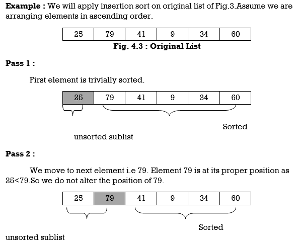
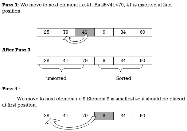
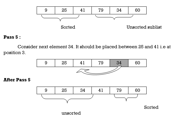
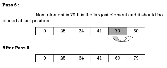
Hence the list is sorted using insertion sort.
We will see one more example.
Apply Insertion sort on array A= {77,30,40,10,88,20,65,56}
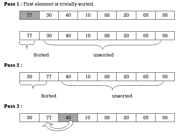
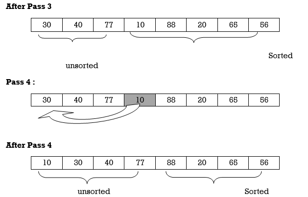

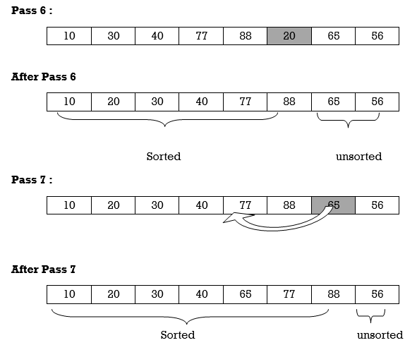
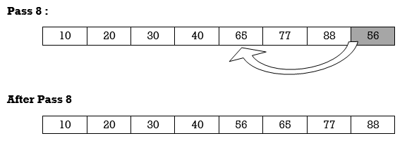
Hence the list is sorted using Insertion sort.
Algorithm:
Algorithm: Insertion-Sort (A)
For j = 2 to A.length
Key = A[j]
// Insert A[j] into the sorted sequence A[1.. j - 1]
i = j - 1
While i > 0 and A[i] > key
A[i + 1] = A[i]
i = i -1
A[i + 1] = key
Analysis:
This algorithm's run time is very dependent on the input given.
If the numbers given are sorted, this algorithm runs in O(n) time. If the numbers given are in reverse order, the algorithm runs in O(n2) time.
Example:
Using insertion sort to sort the following list of elements:
89, 45, 68, 90, 29, 34, 17
89 |45 68 90 29 34 17
45 89 |68 90 29 34 17
45 68 89 |90 29 34 17
45 68 89 90 |29 34 17
29 45 68 89 90 |34 17
29 34 45 68 89 90 |17
17 29 34 45 68 89 90
Complexity of Insertion Sort:
Worst Case Complexity: In the worst case, for each i we do (i – 1) swaps inside the inner for–loop–therefore, overall number of swaps (when i goes from 2 to n in the outer for loop) is
T(n) =1 + 2 + 3 +...+(I – 1) +.... + n – 1
=n (n – 1)/2
=O(n2)
Average case Complexity is O(n2).
Best Case Complexity is O(n).
Application:
In the following instances, the insertion sort algorithm is used:
- When only a few elements are in the list.
- When there are few elements for sorting.
Advantages:
- Straightforward implementation. Three variants exist.
● Left to right scan
● Right to left scan
● Binary insertion sort
2. Effective on a small list of components, on a nearly sorted list.
3. In the best example, running time is linear.
4. This algorithm is stable.
5. Is the on-the-spot algorithm
Key takeaways
Insertion sorting is a very basic process for sorting numbers in an ascending or descending order.
Insertion style is a decrease & conquer technique application.
It is a sort based on comparison in which the sorted array is constructed on one entry at a time.
Heap Sort is one of the best in-place sorting strategies with no worst-case quadratic runtime. Heap sort requires the creation of a Heap data structure from the specified array and then the use of the Heap to sort the array.
You should be wondering how it can help to sort the array by converting an array of numbers into a heap data structure. To understand this, let's begin by knowing what a heap is.
Characteristics
Heap is a unique tree-based data structure that meets the following special heap characteristics:
- Shape property:
The structure of Heap data is always a Complete Binary Tree, which means that all tree levels are fully filled.
2. Heap property:
Every node is either greater or equal to, or less than, or equal to, each of its children. If the parent nodes are larger than their child nodes, the heap is called Max-Heap, and the heap is called Min-Heap if the parent nodes are smaller than their child nodes. It can be classified into two types:
I. Max-Heap
II. Min Heap
Max-Heap: A Max-Heap occurs when the parent nodes are larger than the child nodes.
Min-Heap: A Min-Heap is formed when the parent nodes are smaller than the child nodes.
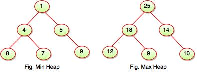
Fig: min and max heap
The Heap sorting algorithm is split into two basic components:
- Creating an unsorted list/array heap.
- By repeatedly removing the largest/smallest element from the heap, and inserting it into the array, a sorted array is then created.
Algorithm
Algorithm
HeapSort(arr)
BuildMaxHeap(arr)
For i = length(arr) to 2
Swap arr[1] with arr[i]
Heap_size[arr] = heap_size[arr] ? 1
MaxHeapify(arr,1)
End
BuildMaxHeap(arr)
BuildMaxHeap(arr)
Heap_size(arr) = length(arr)
For i = length(arr)/2 to 1
MaxHeapify(arr,i)
End
MaxHeapify(arr,i)
MaxHeapify(arr,i)
L = left(i)
R = right(i)
If L ? heap_size[arr] and arr[L] > arr[i]
Largest = L
Else
Largest = i
If R ? heap_size[arr] and arr[R] > arr[largest]
Largest = R
If largest != i
Swap arr[i] with arr[largest]
MaxHeapify(arr,largest)
End
Complexity analysis of heap sort
Time complexity:
Worst case: O(n*log n)
Best case: O(n*log n)
Average case: O(n*log n)
Space complexity: O(1)
Key takeaway:
Heap Sort is one of the best in-place sorting strategies with no worst-case quadratic runtime.
Heap sorting is very fast and for sorting it is widely used.
Heap sorting is not a stable type, and requires constant space to sort a list.
Shell Sort is just an Insertion Sort variant. We just shift elements one position forward in insertion sort. Many moves are required when an element must be pushed far ahead. The goal of shell Sort is to enable for the trading of things from afar. For a big value of h, we use shell Sort to sort the array. We reduce the value of h until it equals one. If all sublists of every h'th element are sorted, the array is said to be h-sorted.
In insertion sort, elements can only be moved forward by one position at a time. Many moves are required to move an element to a far-away point, which increases the algorithm's execution time. Shell sort, on the other hand, eliminates the shortcoming of insertion sort. It also enables for the moving and swapping of far-off elements.
This algorithm sorts the items that are far apart first, then closes the space between them. This space is referred to as an interval. This interval can be determined using Knuth's formula, which is shown below -
Hh = h * 3 + 1
Where, 'h' is the interval having initial value 1.
Algorithm
The simple steps of achieving the shell sort are listed as follows -
ShellSort(a, n) // 'a' is the given array, 'n' is the size of array
For (interval = n/2; interval > 0; interval /= 2)
For ( i = interval; i < n; i += 1)
Temp = a[i];
For (j = i; j >= interval && a[j - interval] > temp; j -= interval)
a[j] = a[j - interval];
a[j] = temp;
End ShellSort
How Shell Sort Works?
Consider the following example to have a better understanding of how shell sort works. We'll use the same array as in the previous examples. For the sake of clarity, we'll use the interval of 4 as an example. Make a virtual sub-list of all values in the four-position interval. 35, 14, 33, 19, 42, 27, and 10, 44 are the figures in this case.
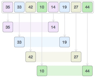
We compare the values in each sub-list and swap them in the original array if necessary. This is how the new array should look after this step:

Then we pick a 1 interval and divide it into two sub-lists: {14, 27, 35, 42} and {19, 10, 33, 44}
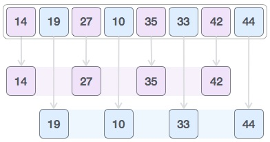
We compare the values in the original array and, if necessary, swap them. This is how the array should look after this step:

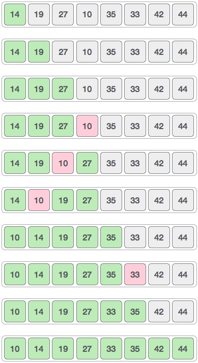
Finally, we use interval 1 to sort the rest of the array. The array is sorted by shell sort using insertion sort.
The following is a step-by-step guide:
Key takeaway
Shell Sort is just an Insertion Sort variant. We just shift elements one position forward in insertion sort. Many moves are required when an element must be pushed far ahead.
A linear or sequential relationship exists when data objects are stored in a collection, such as a list. Each data item is kept in a certain location in relation to the others. These relative positions are the index values of the various items in Python lists. We can access these index values in order because their values are ordered. Our initial searching strategy, the sequential search, is born out of this procedure.
This is how the search works, as shown in the diagram. We just advance from item to item in the list, following the underlying sequential ordering, until we either find what we're looking for or run out of options. If we run out of items, we have discovered that the item we were searching for was not present.

Fig: Sequential search
Algorithm
● LINEAR_SEARCH(A, N, VAL)
● Step 1: [INITIALIZE] SET POS = -1
● Step 2: [INITIALIZE] SET I = 1
● Step 3: Repeat Step 4 while I<=N
● Step 4: IF A[I] = VAL
SET POS = I
PRINT POS
Go to Step 6
[END OF IF]
SET I = I + 1
[END OF LOOP]
● Step 5: IF POS = -1
PRINT " VALUE IS NOT PRESENTIN THE ARRAY "
[END OF IF]
● Step 6: EXIT
Function for Linear search is
Find(values, target)
{
For( i = 0; i < values.length; i++)
{
If (values[i] == target)
{ return i; }
}
Return –1;
}
If an element is found this function returns the index of that element otherwise it returns –1.
Example: we have an array of integers, like the following:

Let’s search for the number 7. According to function for linear search index for element 7 should be returned. We start at the beginning and check the first element in the array.
9 | 6 | 7 | 12 | 1 | 5 |
First element is 9. Match is not found and hence we move to next element i.e., 6.
9 | 6 | 7 | 12 | 1 | 5 |
Again, match is not found so move to next element i.e.,7.
9 | 6 | 7 | 12 | 1 | 5 |
0 | 1 | 2 | 3 | 4 | 5 |
We found the match at the index position 2. Hence output is 2.
If we try to find element 10 in above array, it will return –1, as 10 is not present in the array.
Complexity Analysis of Linear Search:
Let us assume element x is to be searched in array A of size n.
An algorithm can be analyzed using the following three cases.
1. Worst case
2. Average case
3. Best case
1. Worst case: In Linear search worst case happens when element to be searched is not present. When x is not present, the linear search function compares it with all the elements of A one by one. The size of A is n and hence x is to be compared with all n elements. Thus, the worst-case time complexity of linear search would be O(n).
2. Average case: In average case analysis, we take all possible inputs and calculate computing time for all of the inputs. Sum all the calculated values and divide the sum by total number of inputs. Following is the value of average case time complexity.
Average Case Time= ∑= ×= O (n)
3. Best Case: In linear search, the best case occurs when x is present at the first location. So, time complexity in the best-case would-be O (1).
P: Program for Linear Search
#include<stdio.h>
#include<conio.h>
Int search(int [],int, int);
void main()
{
int a[20],k,i,n,m;
Clrscr();
Printf(“\n\n ENTER THE SIZE OF ARRAY”);
Scanf(“%d”,&n);
Printf(“\n\nENTER THE ARRAY ELEMENTS\n\n”);
For(i=0;i<n;i++)
{
scanf(“%d”,&a[i]);
}
printf(“\n\nENTER THE ELEMENT FOR SEARCH\n”);
scanf(“%d”,&k);
m=search(a,n,k);
if(m==–1)
{
printf(“\n\nELEMENT IS NOT FOUND IN LIST”);
}
else
{
printf(“\n\nELEMENT IS FOUND AT LOCATION %d”,m);
}
}
getch();
}
Int search(int a[],int n,int k)
{
int i;
for(i=0;i<n;i++)
{
if(a[i]==k)
{
return i;
}
}
if(i==n)
{
return –1;
}
}
Merits:
- Simple and easy to implement
- It works well even on unsorted arrays.
- It is memory efficient as it does not require copying and partitioning of the array being searched.
Demerits:
- Suitable only for small number of values.
- It is slow as compared to binary search.
Binary Search
Binary search is the search technique which works efficiently on the sorted lists. Hence, in order to search an element into some list by using binary search technique, we must ensure that the list is sorted.
Binary search follows a divide and conquer approach in which the list is divided into two halves and the item is compared with the middle element of the list. If the match is found then, the location of the middle element is returned; otherwise, we search into either of the halves depending upon the result produced through the match.
Binary search algorithm is given below.
BINARY_SEARCH(A, lower_bound, upper_bound, VAL)
Step 1: [INITIALIZE] SET BEG = lower_bound
END = upper_bound, POS = - 1
Step 2: Repeat Steps 3 and 4 while BEG <=END
Step 3: SET MID = (BEG + END)/2
Step 4: IF A[MID] = VAL
SET POS = MID
PRINT POS
Go to Step 6
ELSE IF A[MID] > VAL
SET END = MID – 1
ELSE
SET BEG = MID + 1
[END OF IF]
[END OF LOOP]
Step 5: IF POS = -1
PRINT "VALUE IS NOT PRESENT IN THE ARRAY"
[END OF IF]
Step 6: EXIT
Complexity
SN | Performance | Complexity |
1 | Worst case | O(log n) |
2 | Best case | O(1) |
3 | Average Case | O(log n) |
4 | Worst case space complexity | O(1) |
Example
Let us consider an array arr = {1, 5, 7, 8, 13, 19, 20, 23, 29}. Find the location of the item 23 in the array.
In 1st step:
- BEG = 0
- END = 8ron
- MID = 4
- a[mid] = a[4] = 13 < 23, therefore
In Second step:
- Beg = mid +1 = 5
- End = 8
- Mid = 13/2 = 6
- a[mid] = a[6] = 20 < 23, therefore;
In third step:
- Beg = mid + 1 = 7
- End = 8
- Mid = 15/2 = 7
- a[mid] = a[7]
- a[7] = 23 = item;
- Therefore, set location = mid;
- The location of the item will be 7.
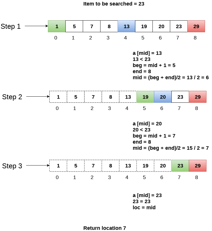
Fig- Example
References:
- Horowitz and Sahani, “Fundamentals of Data Structures”, Galgotia Publications Pvt Ltd Delhi India.
- Lipschutz, “Data Structures” Schaum’s Outline Series, Tata McGraw-hill Education (India) Pvt. Ltd.
- Thareja, “Data Structure Using C” Oxford Higher Education.
- AK Sharma, “Data Structure Using C”, Pearson Education India.